Finding Where a Low-Res Image Came From Inside a High-Res Source

The entire super-resolution field has a data problem that nobody talks about enough. Every SR model trains on synthetic pairs — take a high-res image, run cv2.resize with bicubic interpolation, call the output your “low-resolution” input — and then the paper claims the model learned to enhance real low-res images. It learned to undo bicubic interpolation. That is what it learned. The model has never seen real sensor noise, real lens blur, real compression artifacts, because the training data was manufactured on a laptop.

I spent three months during summer 2022, as part of a CS 497 independent study, building a pipeline to fix this. The idea was straightforward in principle and surprisingly annoying in practice: given a real low-resolution image from one camera and a real high-resolution image from another camera filming the same scene, automatically find the corresponding region in the high-res source and extract a pixel-aligned training pair. The tool that makes this possible is SIFT, an algorithm from 2004 that I initially reached for because it was the boring, obvious choice — and it turned out to be the right one.

The Actual Problem, Stated Precisely

Consider two cameras mounted side by side on a vehicle: a high-resolution DSLR and a low-resolution phone camera. Both point at the same scene. The DSLR captures a 512x512 frame; the phone captures a 100x100 frame that corresponds to roughly a 400x400 region of the DSLR’s field of view, but at 4x lower resolution and from a slightly different position.

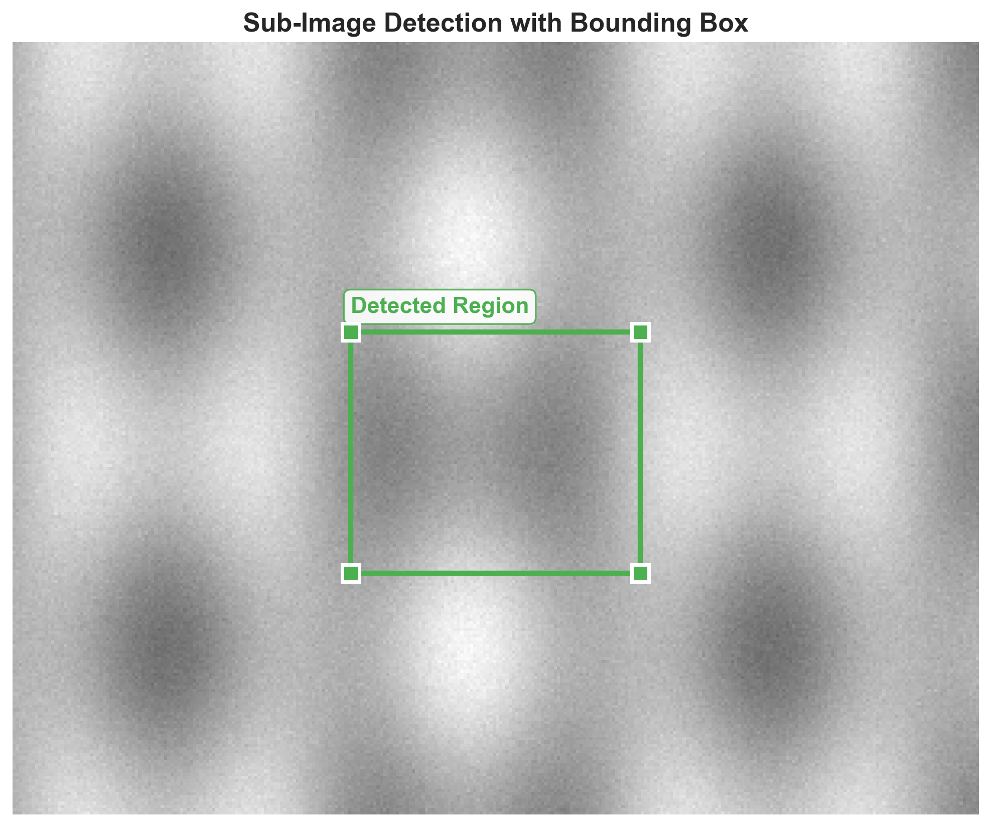
You want the bounding box [x_min, y_min, x_max, y_max] in the high-res image that corresponds to what the low-res camera saw. Once you have that, you can crop the 400x400 region from the DSLR frame, pair it with the 100x100 phone frame, and feed both to a super-resolution model that will learn from real degradation rather than synthetic downsampling.

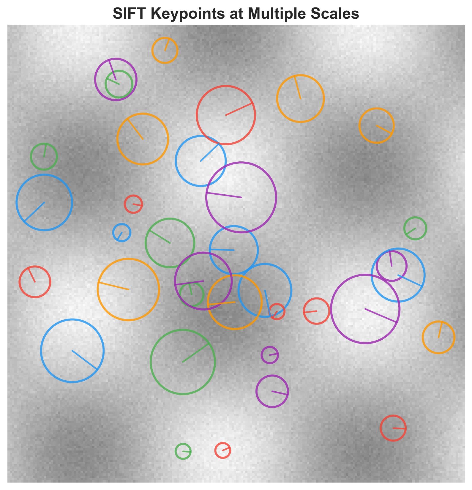
The naive approach — OpenCV’s matchTemplate — fails here because it assumes the template and search image are at the same scale, which they are not. You could do a multi-scale search, but that requires knowing the exact scale factor, and even then the computational cost scales poorly. SIFT features, by contrast, are scale-invariant by definition (that is literally what the S stands for), so a keypoint detected in the 100x100 phone image will have a matching descriptor in the 512x512 DSLR frame regardless of the resolution mismatch.

Feature Extraction and Matching

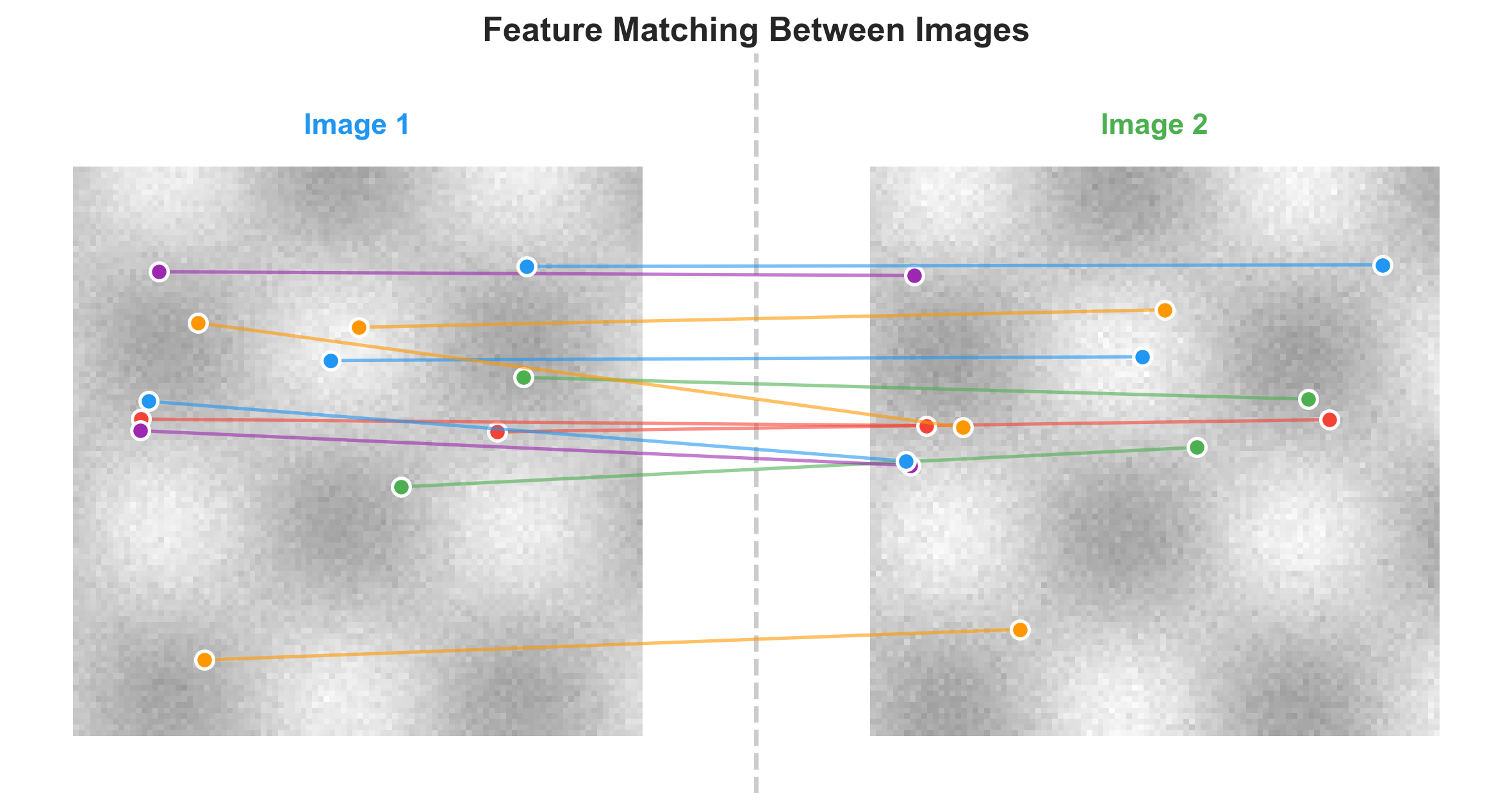
The first stage extracts SIFT keypoints and their 128-dimensional descriptors from both images, then matches them using brute-force search with cross-checking:

def get_match_info(good_image, bad_image):
    good_gray = cv2.cvtColor(good_image, cv2.COLOR_BGR2GRAY)
    bad_gray = cv2.cvtColor(bad_image, cv2.COLOR_BGR2GRAY)

    sift = cv2.xfeatures2d.SIFT_create()

    kp_good, desc_good = sift.detectAndCompute(good_gray, None)
    kp_bad, desc_bad = sift.detectAndCompute(bad_gray, None)

    bf = cv2.BFMatcher(cv2.NORM_L1, crossCheck=True)
    matches = bf.match(desc_good, desc_bad)
    matches = sorted(matches, key=lambda x: x.distance)

    return kp_good, kp_bad, matches

The crossCheck=True parameter means a match only counts if descriptor A’s nearest neighbor is B and B’s nearest neighbor is A. This kills a lot of false positives and costs you some true matches — a trade I found worthwhile after watching the pipeline hallucinate bounding boxes on images with repetitive textures. I went with L1 norm over L2 for the descriptor distance; in my experiments L1 produced slightly more stable results when the scale mismatch was large, though I would not stake my life on the difference being statistically significant.

(The original code has bf = cv2.BFMatcher(cv2.NORM_L1, crossCheck=True) written twice on consecutive lines. I have no explanation for this. I can only assume I was testing something and forgot to delete one.)

From Matches to Bounding Box

Raw SIFT matches give you pairs of corresponding keypoints, but not all of them are geometrically consistent. If the sub-image is a downscaled crop from the source, then the spatial relationship between matched points should be governed by a consistent scale factor. Points that violate this relationship are outliers from repetitive textures or accidental descriptor similarity.

My original filtering was a simplified distance-ratio check rather than full RANSAC:

def remove_bad_matches(good_kp, bad_kp, good_idx, bad_idx, ratio):
    filtered_good, filtered_bad = [], []
    error_margin = 0.05

    for i in range(len(good_kp)):
        distance_good = distance(0, 0, good_kp[i][0], good_kp[i][1])
        distance_bad = distance(0, 0, bad_kp[i][0], bad_kp[i][1])
        distance_ratio = (distance_good * ratio) / distance_bad
        if (1.0 - error_margin) < distance_ratio < (1.0 + error_margin):
            filtered_good.append(good_kp[i])
            filtered_bad.append(bad_kp[i])

    return filtered_good, filtered_bad

The logic: if you know the downscaling ratio is 0.25 (4x downscale), then the distance from the origin to each keypoint in the low-res image should be approximately ratio * distance to the corresponding keypoint in the high-res image. Points that deviate by more than 5% get thrown out. This is crude compared to cv2.findHomography with RANSAC, which I only discovered later — the refactored version of the pipeline uses proper homography estimation, and it handles perspective distortion that my ratio-check approach silently ignores.

From the surviving matches, I find four corner keypoints by computing which matched point in the low-res image is closest to each corner of the axis-aligned bounding box defined by the extremal x and y coordinates:

def get_bottom_left(keys):
    x_min, y_min = get_x_min(keys), get_y_min(keys)
    closest = keys[0]
    min_dist = distance(x_min, y_min, closest[0], closest[1])
    for point in keys:
        d = distance(x_min, y_min, point[0], point[1])
        if d < min_dist:
            closest = point
            min_dist = d
    return closest

Each corner keypoint in the low-res image has a corresponding matched keypoint in the high-res image, so looking up those indices gives you the bounding rectangle in the source. A final validation step checks that the ratio between corresponding coordinates in both windows is consistent — if it is not, the match probably failed and the pipeline skips that image rather than producing garbage training data.

Results and Where It Breaks

I tested the pipeline on Set14, BSD100, and a subset of DIV2K at a 4x downscaling ratio, extracting sub-images at 50x50, 100x100, and 200x200 output sizes. The recovered regions scored 30.8 dB PSNR and 0.84 SSIM against ground truth crops — not pixel-perfect, but the error concentrates at the edges of the bounding box where SIFT keypoints do not land exactly on the image boundary, and for SR training that edge imprecision is tolerable.

The pipeline fails predictably in three cases. Uniform textures like sky regions produce almost no SIFT keypoints, so there is nothing to match. Extreme downscaling ratios (8x or higher) make SIFT descriptors unreliable because the low-res version of a feature patch has lost too much information. And repetitive patterns — brick walls, grids, tiled floors — produce many ambiguous matches that my geometric filtering cannot always resolve. The brick wall failure was the one that convinced me cross-checking was non-negotiable; without it, a brick wall image would produce a confident-looking but completely wrong bounding box.

The 900-Line File

The image_preprocessing/ directory in my CS 497 repo ended up containing 14+ files and something like 900 lines of Python, which is a lot of code for what amounts to “find where this small image lives inside this big image.” Most of that line count came from three months of iterative development: functions that exist because I needed them once during debugging and never deleted them, commented-out print statements from when I was tracing why a particular image produced nonsensical corner coordinates, helper utilities for visualization that I wrote to convince myself the pipeline was working before I automated it. The variable naming alone — good_image, bad_image, good_match_kpl, bad_match_kpindexl — tells you this code was written by someone solving the problem in real time, not someone writing for an audience.

(There are approximately forty blank lines in a row in the middle of the original file. I do not remember why. I suspect I was using whitespace as a section divider, which is the kind of organizational strategy that feels perfectly reasonable at 2 AM and completely unhinged in the morning.)

The refactored version separates detection, matching, localization, and visualization into clean modules, uses Lowe’s ratio test instead of my homebrew distance-ratio filter, and delegates to cv2.findHomography for the geometric estimation. The original version works, the refactored version works better, and the three months between them taught me that the difference between “working prototype” and “production pipeline” is mostly error handling and the willingness to delete code that solved yesterday’s problem.

What This Is Actually For

The primary application is what I described at the top: creating SR training datasets from dual-camera setups where both cameras capture the same scene at different resolutions. Mount the two cameras, capture frames, run SIFT matching to find corresponding regions, extract pixel-aligned crops, and train on real degradation patterns instead of synthetic bicubic downsampling. The same technique works for unpaired dataset alignment — matching low-res images of unknown provenance to their high-res counterparts — and for image forensics, where you want to determine where a cropped region came from within a larger photograph.

SIFT is a 2004 algorithm. There are learned feature matchers now — SuperPoint, SuperGlue, LightGlue — that would handle the textureless and repetitive-pattern failure cases better than SIFT does, at the cost of needing a GPU and substantially more setup. For this specific problem, where the primary challenge is scale invariance and the images are natural scenes with reasonable feature density, the 18-year-old algorithm worked. I wrote a research paper about it (5 pages, 18 references) and moved on to the next thing, and the lesson I took away was not about SIFT specifically but about the value of reaching for the well-understood tool before the impressive one.