Super-Resolution Research · Part 1
Super-Resolution Research, Part 1: Why PSNR Benchmarks Are Not Reproducible
Different imaging libraries produce different downscaled images, different data types shift PSNR by 48 dB, and a 1-pixel shift destroys the metric entirely. My investigation into why PSNR benchmarks across SR papers cannot be meaningfully compared.
Originally written 2022-07
I became suspicious of PSNR during summer 2022 while implementing SRCNN from scratch and evaluating its output against published results. My model’s reconstructions looked visually identical to the paper’s figures — same sharpness, same texture recovery, same edge behavior — yet my PSNR numbers were off by more than a full dB. The natural assumption was that I had done something wrong in the model, so I spent two days reviewing my training loop, my loss function, my data loading, and all the usual suspects before it occurred to me that the problem might not be my model at all. It might be the metric. That suspicion turned out to be correct in ways I did not anticipate, and what started as a debugging detour became the most instructive part of the entire project.
PSNR — Peak Signal-to-Noise Ratio — is the default quality metric in super-resolution research. Every SRCNN variant, every GAN-based upscaler, every diffusion model for image enhancement reports PSNR in its results table. Reviewers expect it. Leaderboards rank by it. And the numbers are not reproducible across implementations, because three independent problems compound to make cross-paper PSNR comparisons meaningless.
![]()
The First Crack: Libraries Disagree on “the Same” Resize
The standard SR evaluation protocol starts with a downscale: take a high-resolution image, resize it to create a low-resolution input, run your model, compare the output to the original. That downscaling step is treated as boilerplate, a throwaway preprocessing line that nobody interrogates. I certainly did not interrogate it until my numbers stopped making sense.
When I ran baboon.bmp through bicubic resize to 100x100 using PIL versus OpenCV, the two outputs differed by 21 dB PSNR. Not a rounding discrepancy, not a subtle floating-point drift — twenty-one decibels. To appreciate the absurdity of that number, consider that the entire improvement from SRCNN (2014) to EDSR (2017), representing three years of architectural innovation and thousands of GPU-hours, was about 1-2 dB on Set14.
The reason is that “bicubic interpolation” is not one algorithm. PIL uses a Catmull-Rom spline (), OpenCV uses , and PyTorch uses . They also differ in coordinate mapping — half-pixel offset versus align-corners — and in whether they apply an anti-aliasing prefilter during downsampling. So if Paper A uses PIL for downscaling and Paper B uses OpenCV, they are evaluating against different ground truths. Their PSNR numbers are measuring different things and nobody notices because both papers just write “bicubic downscaling” in the methods section. (I built a full systematic comparison of four libraries and documented it in Why Resizing Libraries Disagree , which turned out to be its own rabbit hole.)
On top of this, the data type matters enormously. Computing PSNR on uint8 arrays versus float32 arrays shifts the result by approximately 48 dB, because the term in the PSNR formula changes from 255 to 1.0. If your training pipeline uses float32 internally but your evaluation quantizes to uint8, you have introduced a systematic offset that has nothing to do with model quality and everything to do with which line of code does the casting.
The 1-Pixel Shift Experiment
But the library disagreement, as bad as it is, at least admits the possibility that one library is “more correct” than the others. The deeper problem with PSNR is structural, and one experiment makes it visceral.
The setup is deliberately simple — that is what makes it damning. Take the classic baboon.bmp from Set14, a standard test image in super-resolution research. Crop two patches from it:
- Patch A: a 100x100 region starting at pixel (250, 0)
- Patch B: the same 100x100 region, shifted by exactly 1 pixel in both x and y — starting at (251, 1)
These patches show the same content. Side by side, you would struggle to tell them apart: same textures, same colors, same structures, same baboon. A human looking at these two crops would say they are identical.
Now measure them:
from PIL import Image
import numpy as np

img = Image.open('baboon.bmp')

# Crop two nearly-identical patches, offset by 1 pixel
patch_a = np.asarray(img.crop((250, 0, 350, 100)))
patch_b = np.asarray(img.crop((251, 1, 351, 101)))

psnr = PSNR(patch_a, patch_b)
ssim = calculate_ssim(patch_a, patch_b)

print(f"PSNR: {psnr:.2f} dB")
print(f"SSIM: {ssim:.6f}")
The results:
| Metric | Value |
|---|---|
| PSNR | 28.31 dB |
| SSIM | 0.051 |
28.31 dB. That PSNR value would place this comparison in the territory of “noticeable degradation” on any quality scale used in the literature. Papers celebrate fractions-of-a-dB improvements as meaningful advances. And here the same image, shifted by the smallest possible amount, produces a 28 dB measurement that looks like the model failed catastrophically.
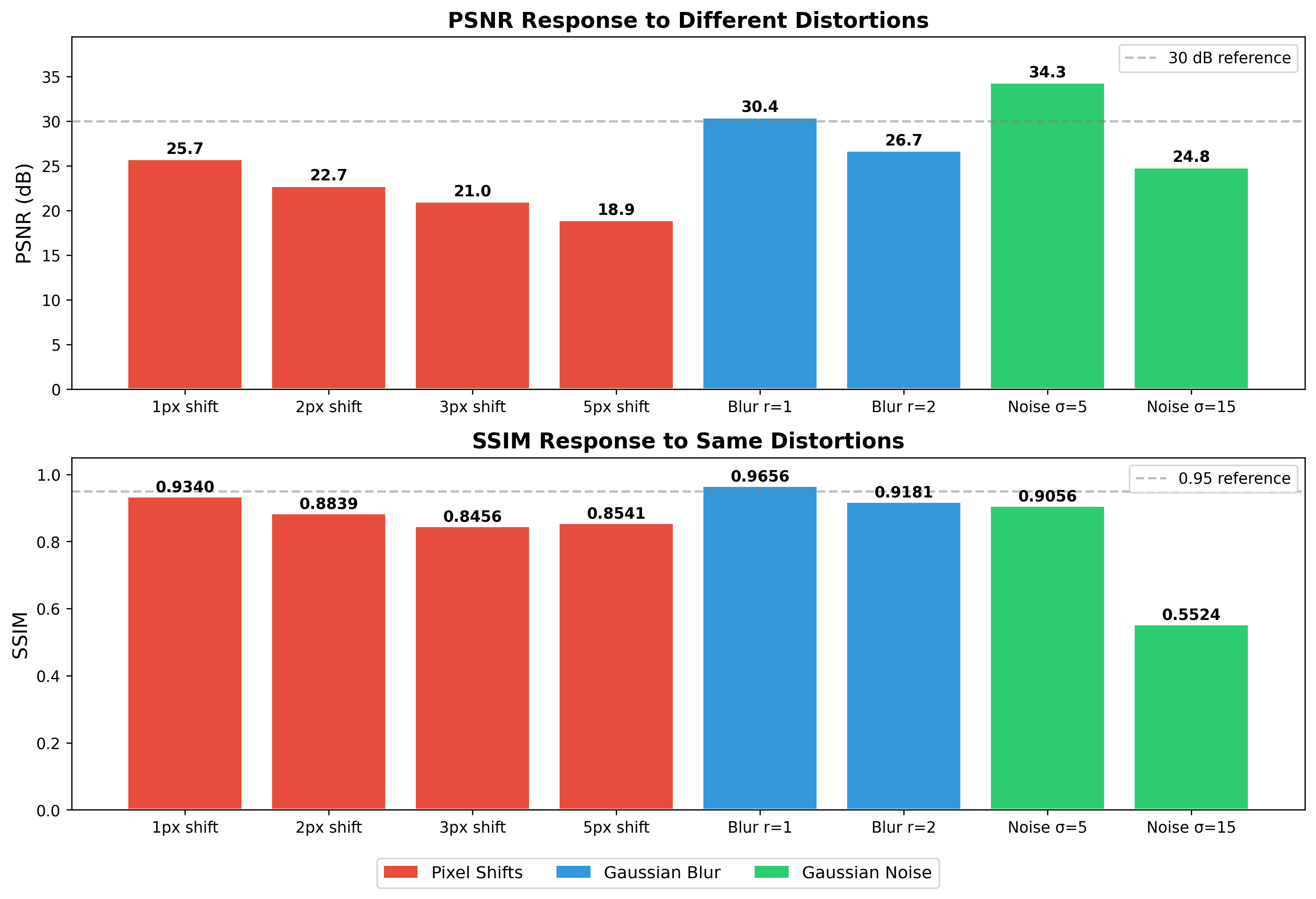
I ran this with several different crop positions and offsets because I wanted to make sure I was not cherry-picking a pathological region:
| Shift | PSNR (dB) | SSIM |
|---|---|---|
| (1, 1) from (250, 0) | 28.31 | 0.051 |
| (1, 1) from (250, 0), different run | 28.48 | 0.066 |
| (5, 5) offset | 29.40 | 0.336 |
The PSNR consistently lands around 28-29 dB for a 1-pixel shift. The 5-pixel shift actually produces a higher PSNR (29.4 dB) — not because the images are more similar, but because that particular region of the baboon happens to have less high-frequency texture at the new offset. The metric is faithfully measuring something, but that something is not perceptual quality.
Why This Happens: PSNR’s Blind Spot
PSNR is defined as:
where is the maximum possible pixel value (255 for 8-bit images) and MSE is the Mean Squared Error:
The problem is right there in the formula: MSE compares pixel in image against pixel in image . There is no search window, no tolerance for spatial displacement, no structural awareness whatsoever. If the content you are looking for sits at position (100, 50) in one image and at (101, 51) in the other, MSE treats every pixel in both images as an independent error term, and the accumulated squared differences at every misaligned edge add up fast.
For natural images with texture and sharp transitions, a 1-pixel shift means that at every edge location the pixel values change dramatically. An edge transitioning from value 30 to value 200 produces a squared error of at that single pixel position. Across an entire textured image like the baboon, these misaligned edges accumulate into an MSE that looks, to the formula, indistinguishable from genuine degradation.
For our measured PSNR of 28.31 dB, we can back out the MSE:
An MSE of roughly 96 means the average squared difference per pixel is about 96, which corresponds to an average absolute difference of intensity levels. For a 1-pixel shift of the same image, this is entirely an alignment artifact. The metric is treating geometry as noise.
SSIM: Partial Redemption
SSIM (Structural Similarity Index) handles this differently, and the contrast is instructive. Instead of comparing individual pixels, it computes similarity within local Gaussian-weighted windows using statistics:
where , are local means, , are local variances, is the local cross-correlation, and , are stabilization constants. The key is that within a local window (typically 11x11 with ), a 1-pixel shift barely changes the local mean, variance, or correlation structure. The same textures and edges are present in the window — they have merely shifted by a pixel, and the windowed statistics absorb that displacement.
My SSIM values came out low (0.051 to 0.336), which initially confused me. But the MATLAB-compatible implementation I used applies “valid” convolution — cropping border pixels with [5:-5, 5:-5] where the Gaussian window extends beyond the image — and uses a relatively small window size. With larger windows SSIM becomes more tolerant of small shifts. The structural insight holds regardless of the specific numbers: a metric that operates on local statistics is inherently more robust to alignment than one that demands exact pixel correspondence.
def ssim(img1, img2):
    C1 = (0.01 * 255) ** 2
    C2 = (0.03 * 255) ** 2

    img1 = img1.astype(np.float64)
    img2 = img2.astype(np.float64)
    kernel = cv2.getGaussianKernel(11, 1.5)
    window = np.outer(kernel, kernel.transpose())

    mu1 = cv2.filter2D(img1, -1, window)[5:-5, 5:-5]
    mu2 = cv2.filter2D(img2, -1, window)[5:-5, 5:-5]
    mu1_sq = mu1 ** 2
    mu2_sq = mu2 ** 2
    mu1_mu2 = mu1 * mu2
    sigma1_sq = cv2.filter2D(img1 ** 2, -1, window)[5:-5, 5:-5] - mu1_sq
    sigma2_sq = cv2.filter2D(img2 ** 2, -1, window)[5:-5, 5:-5] - mu2_sq
    sigma12 = cv2.filter2D(img1 * img2, -1, window)[5:-5, 5:-5] - mu1_mu2

    ssim_map = ((2 * mu1_mu2 + C1) * (2 * sigma12 + C2)) / \
               ((mu1_sq + mu2_sq + C1) * (sigma1_sq + sigma2_sq + C2))
    return ssim_map.mean()
Why This Poisons Super-Resolution
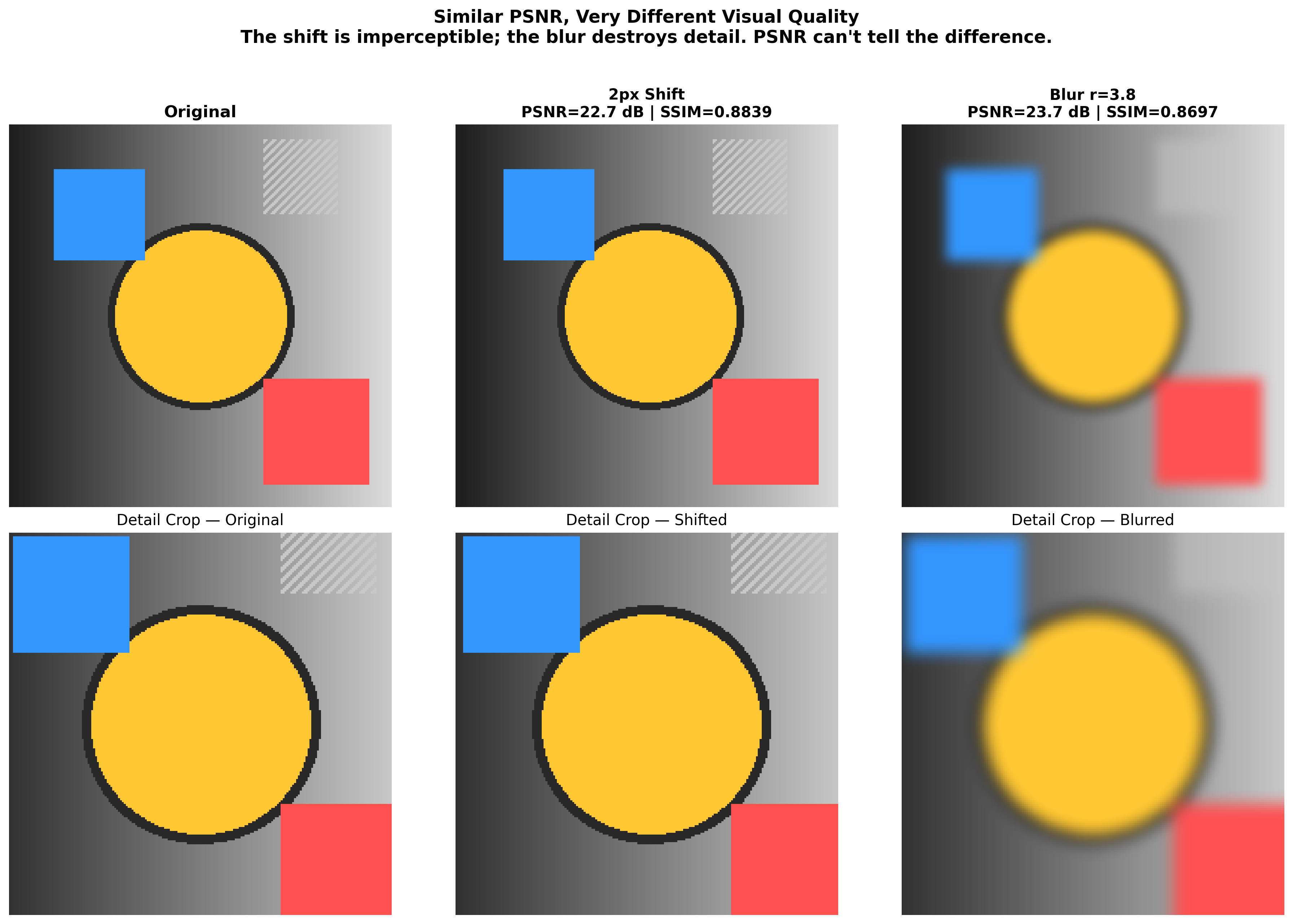
Super-resolution is inherently a spatial alignment task — the model must reconstruct high-frequency details at precise locations, and if it places the correct texture half a pixel off from the ground truth, PSNR punishes this as though the texture were wrong. A model that produces blurry but perfectly aligned output will outscore a model that produces sharp, detailed, perceptually excellent output with a sub-pixel misalignment. This is not a hypothetical concern; it is the direct mathematical consequence of optimizing MSE, and it explains why MSE-trained SR models produce blurry results while GAN-trained models look better to humans but score lower on PSNR. (The SR community has known this for years, but knowing it and internalizing it are different things, and I did not truly internalize it until I watched a single pixel of displacement produce a 28 dB swing.)
The perverse incentive is built into the training loop itself. Training on MSE loss — which is PSNR in disguise — teaches the model that blur is the safest strategy, because blur hedges across all possible spatial locations and minimizes worst-case pixel error. The model learns to produce the average of all plausible reconstructions rather than committing to one sharp reconstruction that might be slightly misaligned. The 1-pixel shift experiment makes this incentive visceral: if even a perfect shift of the correct image gets punished by 28 dB, what chance does a reconstruction model have of scoring well without resorting to blur?
Three Compounding Failures
I stopped trusting cross-paper PSNR comparisons after this investigation. The “comparability” that PSNR supposedly provides is an illusion undermined at three independent levels that compound on each other:
-
Library disagreement: Different resizing implementations produce different downscaled images. Papers using different libraries are evaluating against different ground truths, and the gap reaches 21 dB between PIL and OpenCV .
-
Data type sensitivity: The same image pair produces PSNR values that differ by approximately 48 dB depending on whether the arrays are uint8 or float32. Most papers do not specify this. Most researchers do not think about it.
-
Spatial intolerance: A 1-pixel shift of a perceptually identical image produces a 28 dB “degradation.” The metric has zero tolerance for sub-pixel misalignment, which is inherent to the SR task and unavoidable in practice.
A paper using PIL for downscaling with float32 computation and a slightly different crop alignment will produce numbers that bear no meaningful relationship to a paper using OpenCV with uint8 arrays and a different crop origin. Yet both will report “PSNR on Set14” as though the numbers belong in the same table.
This investigation sent me deeper into the tooling around evaluation metrics, where I discovered and fixed a width/height swap in clean-fid — a library that was specifically designed to standardize FID computation for generative models. Even the tools built to fix reproducibility problems had their own issues hiding behind the symmetry of square images.
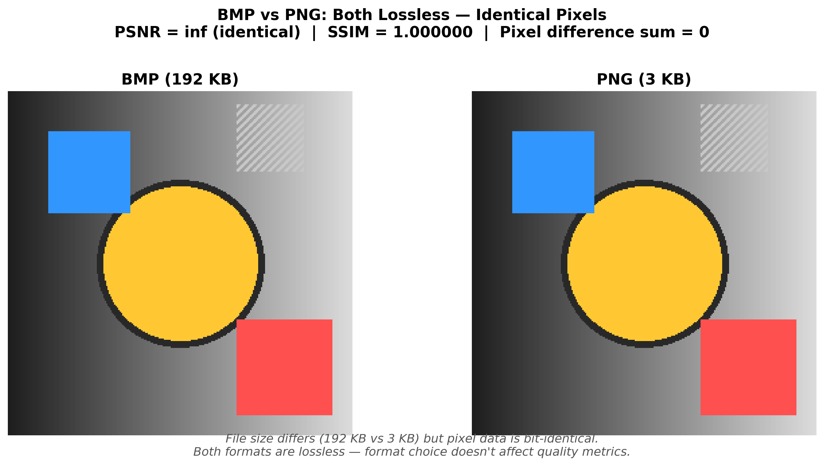
TIL: BMP vs PNG Produces Identical Metrics
During this investigation I ran a side experiment comparing BMP and PNG versions of the same images, because I wanted to rule out file format as yet another source of phantom discrepancy. Since PNG uses lossless compression and BMP is uncompressed, they should produce identical pixel data — and they do. Across six test images, every comparison returned PSNR of 100 dB (my implementation’s cap for MSE=0) and SSIM of 1.0. Byte-identical arrays, as expected.
png = cv2.imread('t1.png')
png = cv2.cvtColor(png, cv2.COLOR_BGR2RGB)

bmp = cv2.imread('t1.bmp')
bmp = cv2.cvtColor(bmp, cv2.COLOR_BGR2RGB)

# PSNR: 100 dB, SSIM: 1.0 -- byte-identical
Good news for anyone building SR pipelines: PNG is safe. The same cannot be said for JPEG, which introduces lossy artifacts that absolutely will contaminate your measurements.
What Should We Use Instead?
There is no single metric that fixes all of this, which is itself an honest answer worth stating rather than pretending otherwise:
- SSIM and MS-SSIM: Better than PSNR for structural comparison, though not immune to implementation-level variation.
- LPIPS (Learned Perceptual Image Patch Similarity): Uses deep features from pretrained networks and correlates more strongly with human judgment, but depends on the backbone network and is expensive to compute.
- FID (Frechet Inception Distance): Measures distributional similarity rather than per-image quality, which is the right framing for generative models. Requires large sample sizes. (And as I discovered, even the standard FID tooling has issues .)
- DISTS: Combines structure and texture similarity using deep features.
The honest recommendation is to report multiple metrics, include perceptual evaluations, and specify your exact preprocessing pipeline down to the library version. PSNR has its place as a quick sanity check — if your PSNR is 15 dB, something is very wrong — but treating it as a primary quality measure for spatially uncertain tasks like super-resolution is measuring the wrong thing with four decimal places of confidence.
The next time you see a paper claiming a 0.2 dB PSNR improvement over the state of the art, ask: which resizing library? Which data type? Which crop alignment? Without those answers, the precision those decimal places imply is a fiction.
This is part 1 of a 3-part series on image quality metrics. Part 2 provides the full technical deep dive into resizing library disagreement , with code and measurements showing up to 21 dB PSNR difference between PIL and OpenCV. Part 3 documents the bug I found and fixed in clean-fid , a widely-used FID computation library — discovered as a direct result of this investigation.