Building Deep Learning from Scratch · Part 2
Building Deep Learning from Scratch, Part 2: A Neural Network in 60 Lines of NumPy
I built a two-layer neural network from scratch using only NumPy, trained it on MNIST, and hit 87.7% accuracy. No frameworks, no autograd — just matrix math and manually derived gradients.
Originally written 2022-12
There is a difference between understanding how neural networks work and actually building one. I had read the backpropagation chapter in Goodfellow’s deep learning textbook, watched the 3Blue1Brown series twice, and could recite the chain rule in my sleep, but I still could not tell you exactly what shape dW1 should be or why dividing pixel values by 255 is the difference between a working network and a screen full of NaN. So in December 2022, I sat down and wrote the whole thing from scratch — forward pass, backward pass, gradient descent — in about 60 lines of NumPy, trained it on 42,000 handwritten digits, and got 87.7% accuracy on the training set.
This post walks through that implementation. I also wrote a companion paper, “Neural Networks From Scratch: The Core Mathematics,” that derives every gradient in formal detail, but the code-first version is what actually taught me the mechanics.
The Architecture
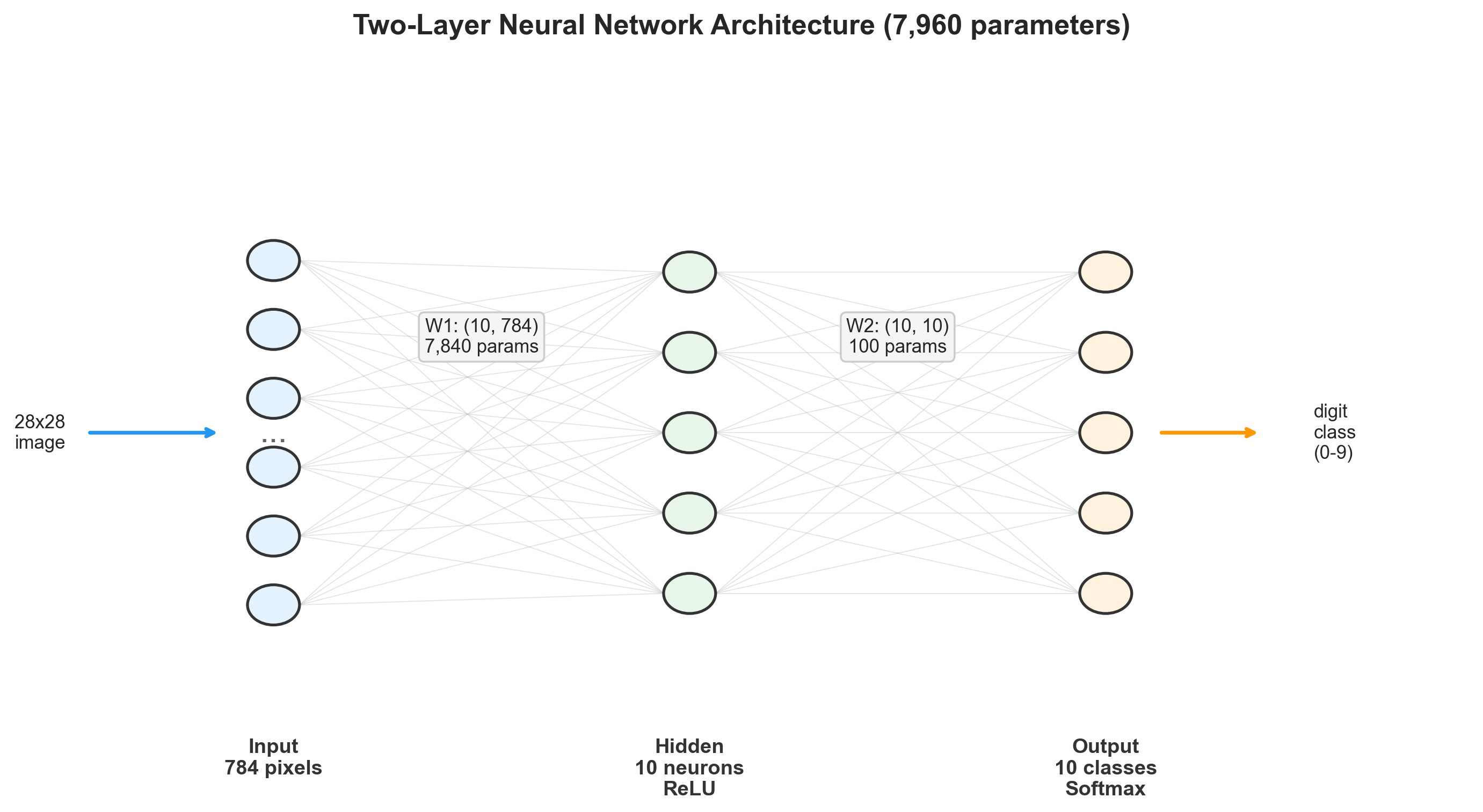
The network is deliberately minimal: two fully connected layers, 7,960 total parameters, and nothing clever about any of it.
The input layer takes 784 values (one per pixel in a 28x28 grayscale image), the hidden layer has 10 neurons with ReLU activation, and the output layer has 10 neurons with softmax — one per digit class. The parameter count breaks down like this:
| Parameter | Shape | Count |
|---|---|---|
| 7,840 | ||
| 10 | ||
| 100 | ||
| 10 | ||
| Total | 7,960 |
I chose 10 hidden neurons because I wanted the bottleneck to be severe. With only 10 dimensions to work with, the hidden layer has to compress 784 pixels down to something that still carries enough information to distinguish a 3 from an 8. A larger hidden layer would push accuracy well above 95%, but it would also let me get away with not understanding the geometry of what the network was learning. The constraint was the point.
Getting the Data Right
MNIST arrives as a CSV: each row is a flattened 28x28 image with a label column up front. The preprocessing is three operations, and two of them taught me something I did not expect.
import numpy as np
import pandas as pd

pd_data = pd.read_csv('./mnist_data/train.csv')
np_data = np.array(pd_data)
rows, cols = np_data.shape
np.random.shuffle(np_data)

# Split: 1000 test, 41000 train
test_data = np_data[0:1000].T
y_test = test_data[0]
x_test = test_data[1:] / 255.0

train_data = np_data[1000:].T
y_train = train_data[0]
x_train = train_data[1:] / 255.0
The transpose. I transpose the data so each column is one example and each row is one feature. This seems like a trivial bookkeeping decision, but it makes all the matrix math downstream fall into place: multiplies weights by examples and produces activations in the same column-per-example layout. After transposing, x_train.shape is (784, 41000) — 784 pixels by 41,000 images. I spent an embarrassing amount of time on shape errors before settling on this convention, and then everything clicked.
Normalization. Pixel values get divided by 255 to map from to . I learned why this matters the hard way: without it, the raw pixel values are large enough that the exponentials in softmax overflow, the weight updates explode, and you get NaN by iteration 3. This was my first real debugging session on the project — I stared at the training output, saw accuracy flatline at 10% (random chance for 10 classes), added a print statement inside softmax, and found inf values. The fix was one line. The lesson stuck.
One-hot encoding. The targets need to become vectors — a label of 7 becomes [0,0,0,0,0,0,0,1,0,0]:
def one_hot_encode(y):
    one_hot_y = np.zeros((y.size, y.max() + 1))
    one_hot_y[np.arange(y.size), y] = 1
    one_hot_y = one_hot_y.T
    return one_hot_y
That indexing trick with np.arange(y.size) and y sets the correct position to 1 for all examples simultaneously — no loop required. I originally wrote a loop. It was slow. NumPy’s fancy indexing is one of those features where reading the documentation pays for itself within the hour.
Forward Pass
The forward pass is four lines of math, which is part of what makes this project satisfying: you can hold the entire computation in your head.
def ReLU(Z):
    return np.maximum(Z, 0)

def softmax(Z):
    A = np.exp(Z) / sum(np.exp(Z))
    return A

def forward_propagation(W_1, b_1, W_2, b_2, X):
    Z_1 = W_1.dot(X) + b_1
    A_1 = ReLU(Z_1)
    Z_2 = W_2.dot(A_1) + b_2
    A_2 = softmax(Z_2)
    return Z_1, A_1, Z_2, A_2
ReLU is np.maximum(Z, 0) — element-wise, trivial to differentiate, and it introduces the nonlinearity that prevents the whole network from collapsing into a single linear transformation. Without it, stacking two matrix multiplications is mathematically equivalent to one.
The softmax implementation has a detail that cost me about two hours. Notice that sum(np.exp(Z)) uses Python’s built-in sum, not np.sum. On a 2D array, Python’s sum operates along axis 0 (columns), producing a row vector that broadcasts correctly when you divide. If you use np.sum instead, it collapses everything into a single scalar, and every probability comes out identical. The predictions looked “reasonable” at a glance — they were all around 0.1, which is plausible for a 10-class problem — so it took me a while to realize the network wasn’t actually learning anything. (The probability for every class was just because the denominator was the sum over all examples, not each one individually.)
For a batch of examples, the dimensional flow looks like this:
| Quantity | Shape | Description |
|---|---|---|
| Input | ||
| Layer 1 weights | ||
| Pre-activation | ||
| Post-activation | ||
| Layer 2 weights | ||
| Pre-activation | ||
| Output probabilities |
Each column of is a probability distribution over the 10 digit classes for one image.
Backward Pass: Where the Real Work Is
The forward pass is mechanical. The backward pass is where I actually had to sit with a pencil and derive things. The goal: compute the gradient of the loss with respect to every parameter, so we know which direction to push the weights.
The loss is implicitly the cross-entropy between the softmax output and the one-hot targets. I say “implicitly” because we never compute the loss value itself during backprop — we jump straight to its gradient, which has a beautiful closed-form expression.
The Output Layer
The combined derivative of softmax + cross-entropy simplifies to:
This is genuinely one of the most satisfying results in the whole derivation. The gradient at the output is just the difference between what the network predicted and what it should have predicted. No chain rule gymnastics, no Jacobian of the softmax — it all cancels out. I spent a full evening working through the derivation by hand (it is in the companion paper), and when I arrived at , I did not believe it at first. I re-derived it twice.
Layer 2 Weight and Bias Gradients
The averages over all 41,000 examples. Without it, the gradients scale linearly with batch size and you have to adjust the learning rate whenever you change the number of training examples.
Propagating Back Through Layer 1
where is element-wise multiplication and .
def derivative_ReLU(Z):
    return Z > 0  # boolean array: True=1, False=0
This is a nice NumPy trick: the comparison Z > 0 produces a boolean array that works as 0/1 in arithmetic. The ReLU derivative is 1 where the input was positive, 0 where it was not. The element-wise multiply zeros out the gradient for any neuron that was “off” during the forward pass — those neurons contributed nothing to the output, so their upstream weights get no gradient signal.
Layer 1 Weight and Bias Gradients
The Complete Backward Function
def backward_propagation(Z_1, A_1, Z_2, A_2, W_2, X, Y):
    one_hot_y = one_hot_encode(Y)
    m = Y.size

    dZ_2 = A_2 - one_hot_y
    dW_2 = (1 / m) * dZ_2.dot(A_1.T)
    db_2 = (1 / m) * np.sum(dZ_2)

    dZ_1 = W_2.T.dot(dZ_2) * derivative_ReLU(Z_1)
    dW_1 = (1 / m) * dZ_1.dot(X.T)
    db_1 = (1 / m) * np.sum(dZ_1)

    return dW_1, db_1, dW_2, db_2
Every shape has to match exactly. dZ_2 is , A_1.T is , so dW_2 comes out — same shape as . I checked every intermediate shape with assert statements during development and removed them once things worked. If you are implementing this yourself, keep the asserts in until you are confident.
Parameter Update and Training
Vanilla gradient descent. No momentum, no Adam, no learning rate scheduling. Just subtract.
def update_params(W_1, b_1, W_2, b_2, dW_1, db_1, dW_2, db_2, alpha):
    W_1 = W_1 - alpha * dW_1
    b_1 = b_1 - alpha * db_1
    W_2 = W_2 - alpha * dW_2
    b_2 = b_2 - alpha * db_2
    return W_1, b_1, W_2, b_2
The training loop ties everything together:
def gradient_descent(X, Y, num_iterations, alpha):
W_1, b_1, W_2, b_2 = initialize_params()
for i in range(num_iterations):
Z_1, A_1, Z_2, A_2 = forward_propagation(W_1, b_1, W_2, b_2, X)
dW_1, db_1, dW_2, db_2 = backward_propagation(Z_1, A_1, Z_2, A_2, W_2, X, Y)
W_1, b_1, W_2, b_2 = update_params(
W_1, b_1, W_2, b_2, dW_1, db_1, dW_2, db_2, alpha
)
if i % 10 == 0:
predictions = np.argmax(A_2, axis=0)
accuracy = np.sum(predictions == Y) / Y.size
print(f"Iteration #{i} -- Accuracy: {accuracy:.4f}")
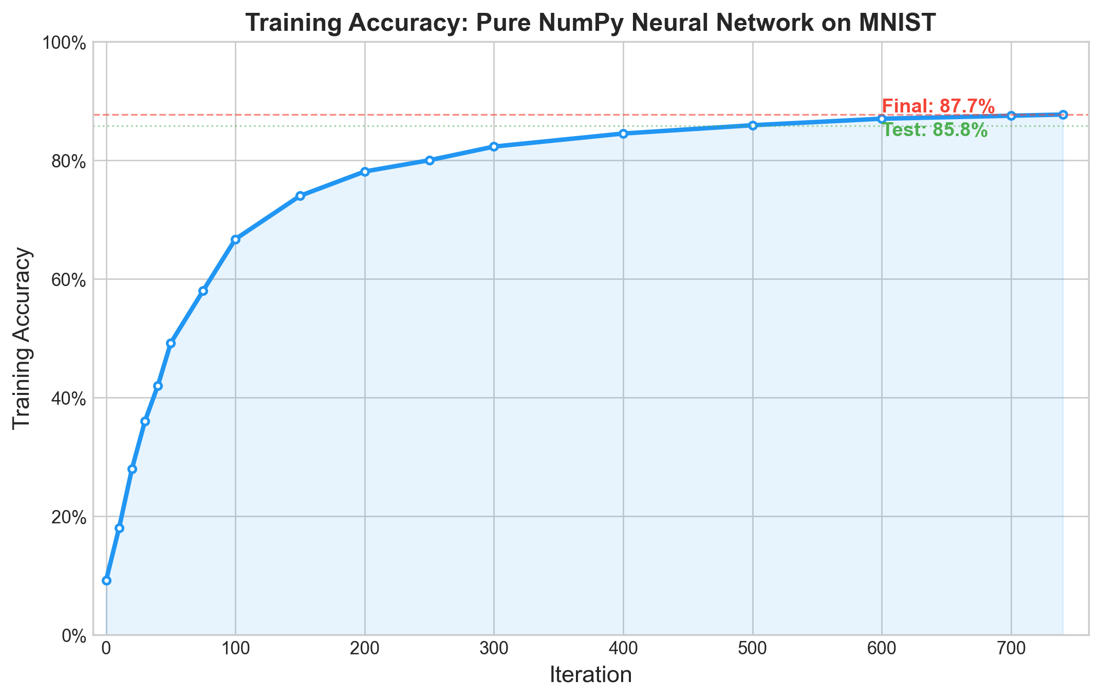
return W_1, b_1, W_2, b_2I trained for 750 iterations at a learning rate of 0.1, which took about 30 seconds on my laptop.
W_1, b_1, W_2, b_2 = gradient_descent(x_train, y_train, 750, 0.1)Results
| Iteration | Accuracy |
|---|---|
| 0 | 9.2% |
| 50 | 49.2% |
| 100 | 66.7% |
| 200 | 78.1% |
| 300 | 82.3% |
| 500 | 85.9% |
| 740 | 87.7% |
The network starts at random-chance accuracy (~10% for 10 classes) and climbs fast in the first 100 iterations, then gradually flattens out. Each subsequent iteration contributes less. This is the textbook learning curve shape, and seeing it emerge from code I wrote myself was more satisfying than any lecture.
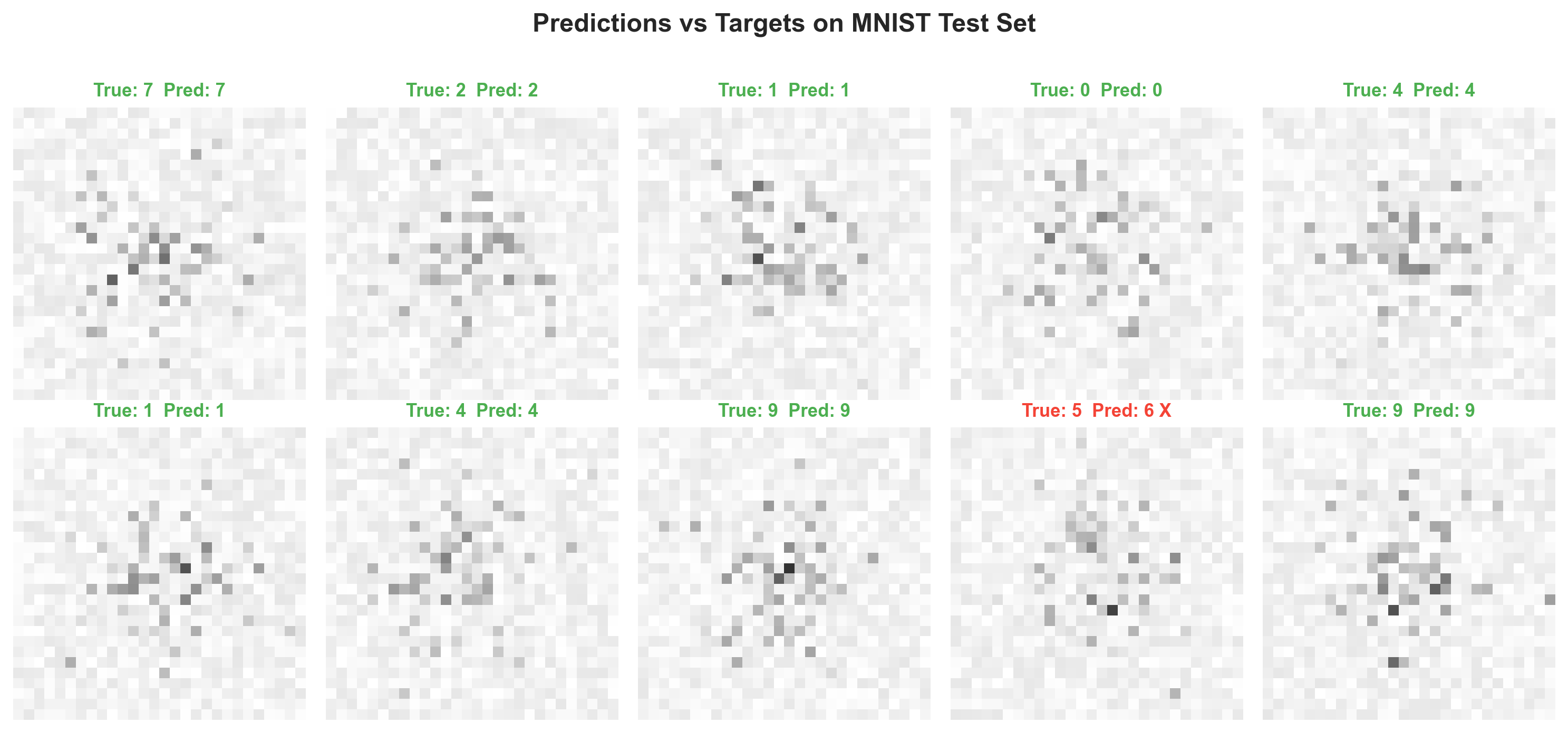
On the held-out test set (1,000 images the network never saw during training):
test_predictions = make_predictions(x_test, W_1, b_1, W_2, b_2)
accuracy = np.sum(test_predictions == y_test) / y_test.size  # => 0.858
Test accuracy: 85.8% — about 2 points below training accuracy, which means the network is not overfitting in any serious way. For a model with no regularization and fewer than 8,000 parameters, that gap is actually encouraging.
Why Not Higher?
State-of-the-art on MNIST exceeds 99.7% with convolutional networks. The 87.7% reflects constraints I chose deliberately:
10 hidden neurons is a severe bottleneck. The network has to compress 784 dimensions into 10, which forces it to learn an extremely compact feature representation. Bumping to 128 hidden neurons would likely break 95%.
No convolutional layers. The fully connected architecture treats every pixel independently. It has no concept of spatial adjacency — it does not know that pixel (5,5) is next to pixel (5,6). CNNs exist precisely to exploit this structure.
Vanilla gradient descent. No momentum, no adaptive learning rates, no scheduling. The optimization literature exists for a reason, and ignoring all of it costs real performance.
Full-batch training. Every iteration processes all 41,000 examples at once, which gives stable gradient estimates but is computationally expensive per step. Mini-batch training (32-256 examples per step) would converge faster in wall-clock time and the noise in the gradient estimates actually helps escape shallow local minima.
The 87.7% is not a failure. It is a demonstration that even the most stripped-down neural network, with no optimization tricks and fewer parameters than some linear models I have seen in production, can learn to read handwriting from raw pixels. The point was never to compete on a leaderboard. The point was to understand every matrix multiply between input and output.
What I Actually Learned
The normalization incident was the most instructive single moment. Training without dividing by 255 produced NaN by the third iteration, and tracking down why — the exponentials in softmax hitting inf, the weight updates blowing up, the whole cascade — taught me more about numerical stability than any textbook section on the topic. Every deep learning practitioner has a normalization war story. This was mine, and it happened on a toy problem with fewer than 8,000 parameters. (I shudder to think about debugging this in a model with millions.)
The sum vs np.sum bug in the softmax was subtler and more annoying. The network “trained” for hundreds of iterations at exactly 10% accuracy, which looked like a learning rate problem or an initialization problem, until I added per-class probability printouts and saw that every class had identical probability. The softmax was normalizing over the wrong axis. It took me most of an evening to find.
The companion paper derives the softmax + cross-entropy gradient in full — the Jacobian of softmax, the chain rule through cross-entropy, the cancellation that produces . That derivation is worth doing once. After you have done it, the clean four-line backward pass starts to feel inevitable rather than mysterious.
Connection to the Micrograd Series
The micrograd implementation and this project represent two complementary ways of understanding neural networks from the ground up:
| Micrograd | NumPy NN | |
|---|---|---|
| Differentiation | Automatic (autograd) | Manual (derived by hand) |
| Data type | Scalars | Matrices |
| Backprop | Generic (works for any computation) | Specific (formulas per layer type) |
| Performance | Educational only | Trains on real data |
Micrograd teaches the mechanism of backpropagation — how gradients flow through a computation graph. The NumPy network teaches the mathematics — what the gradients actually are for specific layer types. Together they provide a complete picture of what happens when you call loss.backward() followed by optimizer.step() in PyTorch.
This implementation is, in miniature, exactly what PyTorch and TensorFlow do behind their APIs. The difference is automatic differentiation, GPU acceleration, and a much richer library of layer types and optimizers. But the core loop — forward, backward, update, repeat — is the same loop. That was the whole point of writing it from scratch.
This post is part of the “Building Deep Learning from Scratch” series. The full source code and companion paper are available in the project repository .