Building Deep Learning from Scratch, Part 1: An Autograd Engine in 80 Lines of Python

I wanted to know what .backward() actually does. Not in the “I read the PyTorch docs” sense — in the “I can write it from memory” sense. So in September 2022, following the general arc of Andrej Karpathy’s micrograd tutorial but writing and reasoning through every line independently, I built a scalar-valued autograd engine from scratch, wrapped it in a small neural network library, and trained a tiny MLP until it converged. The whole engine is about 80 lines of Python, and by the end of the project I could explain reverse-mode automatic differentiation without reaching for an analogy, which was the entire point.

This post covers the full arc: from computing derivatives by hand, through the Value class and its backward functions, to the training loop that ties it all together. It started as a three-part series, but the pieces are better read as one continuous narrative, because the bugs and wrong turns in part one inform the design decisions in part three.

Starting with a Nudge

Before building any machinery, I wanted to ground myself in what a derivative actually is at the computational level. Not the calculus definition — the operational one. Consider:

$$f(x) = 3x^2 - 4x + 5$$

The derivative at any point can be approximated by bumping the input and measuring how the output changes:

def f(x):
    return 3*x**2 - 4*x + 5

h = 0.00000001
x = 2/3
(f(x + h) - f(x)) / h  # => ~0.0

At $x = 2/3$, the analytical derivative is $f'(x) = 6x - 4 = 0$, and the numerical approximation confirms it. This “bump and measure” idea is conceptually the foundation of everything that follows, and I kept coming back to it as a sanity check throughout the project.

The technique extends to multiple inputs. For the expression $d = a \cdot b + c$:

h = 0.0001
a = 2.0; b = -3.0; c = 10.0
d1 = a * b + c

# dd/da: bump a, measure change in d
a += h
d2 = a * b + c
print("dd/da =", (d2 - d1) / h)  # => -3.0 (which is b)

The partial derivative of $d$ with respect to $a$ is $b = -3.0$, with respect to $b$ is $a = 2.0$, and with respect to $c$ is $1.0$. All consistent with the analytical result. But bumping each input one at a time does not scale — a network with 41 parameters (let alone millions) needs a systematic approach. That systematic approach is backpropagation, and to implement it, I needed a data structure that tracks how values are computed.

The Value Class

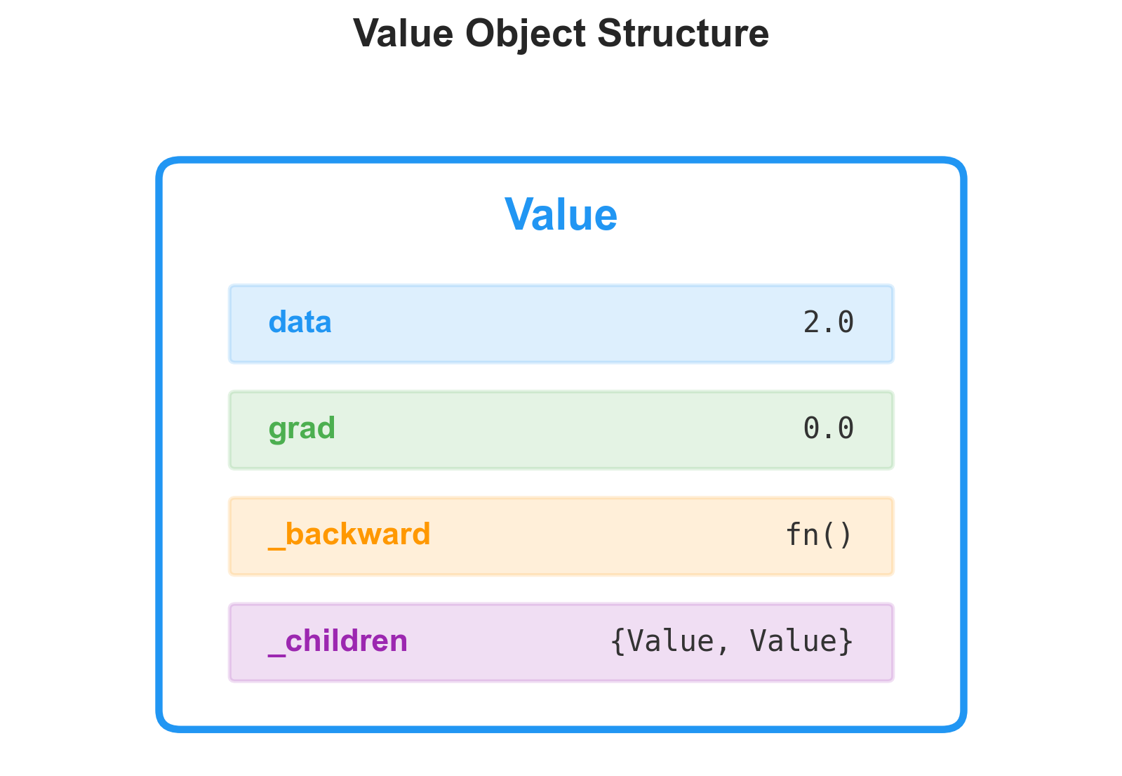
The idea is to wrap every scalar in a Value object that remembers where it came from. Each Value holds its numerical data, a pointer to the child Value objects that produced it, the operation that created it, and a gradient slot that starts at zero:

class Value:

    def __init__(self, data, _children=(), _op=(), label=''):
        self.data = data
        self._prev = set(_children)
        self._op = _op
        self.label = label
        self.grad = 0.0
        self._backward = lambda: None

    def __repr__(self):
        return f"Value(data={self.data})"

    def __add__(self, other):
        other = other if isinstance(other, Value) else Value(other)
        out = Value(self.data + other.data, (self, other), '+')
        return out

    def __mul__(self, other):
        other = other if isinstance(other, Value) else Value(other)
        out = Value(self.data * other.data, (self, other), '*')
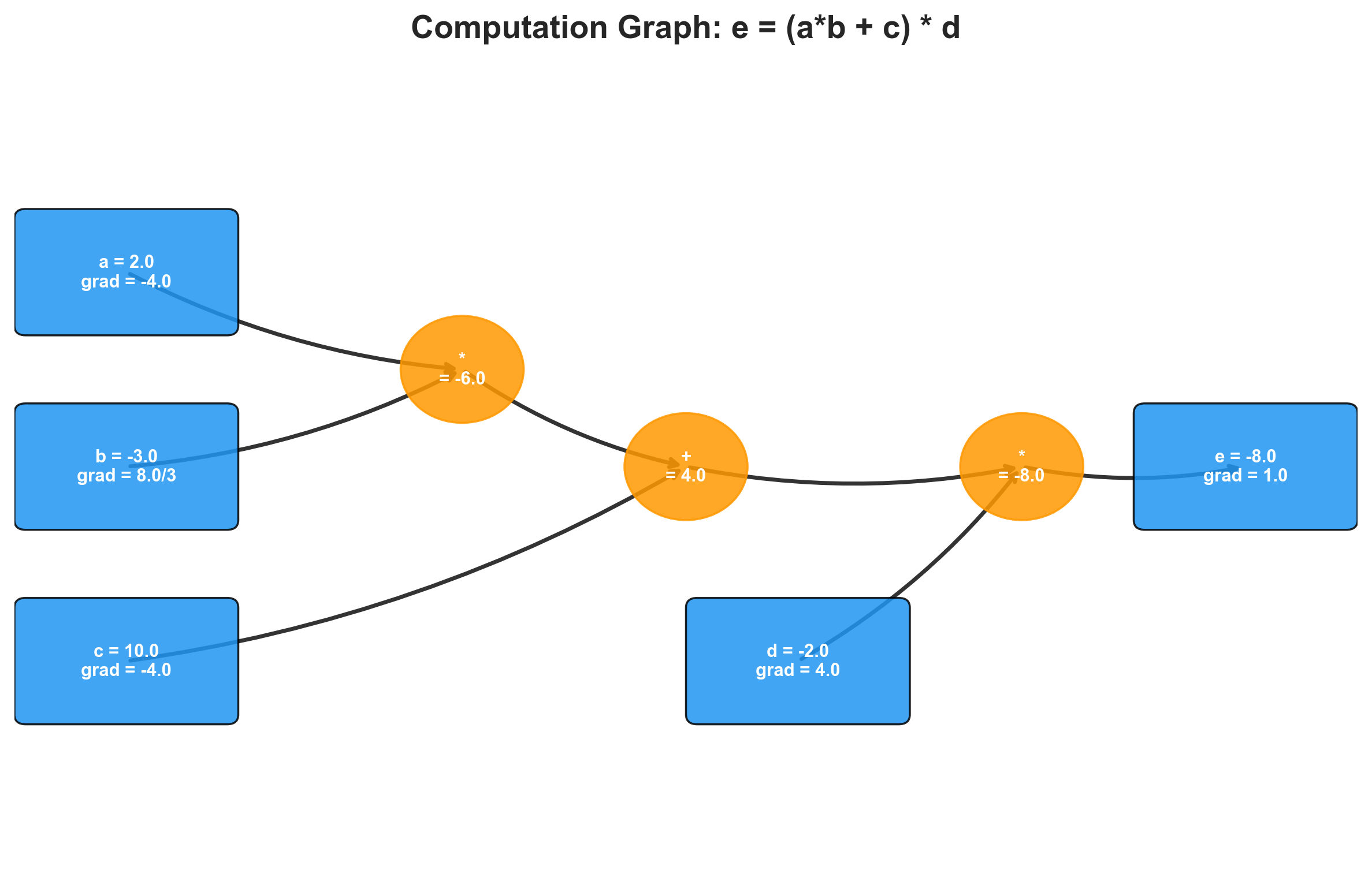
        return out

Every arithmetic operation creates a new Value whose _prev points back to its operands. This implicitly builds a directed acyclic graph — the computation graph. I can set up an expression like $L = (a \cdot b + c) \cdot f$:

a = Value(2.0, label='a')
b = Value(-3.0, label='b')
c = Value(10.0, label='c')
e = a * b; e.label = 'e'
d = e + c; d.label = 'd'
f = Value(-2.0, label='f')
L = d * f; L.label = 'L'

This computes $L = (2 \cdot (-3) + 10) \cdot (-2) = -8$, and every intermediate value remembers its parents.

I used Graphviz to visualize the graph — two helper functions that traverse the DAG and render each node with its data and gradient. Being able to see the computation graph made the rest of the project far more tractable. When a gradient came out wrong, I could look at the picture and trace the error backward through the graph by hand.

Manual Backpropagation

With the graph built, I computed gradients by hand. The chain rule says: for a composition $L = f(g(x))$, the derivative $\frac{\partial L}{\partial x} = \frac{\partial L}{\partial g} \cdot \frac{\partial g}{\partial x}$. In the computation graph, each node receives its gradient from its consumer, multiplied by the local derivative of the operation.

Working through $L = d \cdot f$ where $d = 4.0$ and $f = -2.0$:

$\frac{\partial L}{\partial L} = 1.0$ (the output’s gradient with respect to itself is always 1).

$L = d \cdot f$, so $\frac{\partial L}{\partial d} = f = -2.0$ and $\frac{\partial L}{\partial f} = d = 4.0$.

$d = e + c$, and addition distributes the gradient unchanged: $\frac{\partial L}{\partial e} = -2.0$, $\frac{\partial L}{\partial c} = -2.0$.

$e = a \cdot b$, so $\frac{\partial L}{\partial a} = \frac{\partial L}{\partial e} \cdot b = (-2.0)(-3.0) = 6.0$ and $\frac{\partial L}{\partial b} = \frac{\partial L}{\partial e} \cdot a = (-2.0)(2.0) = -4.0$.

I verified these by nudging each input in the direction of its gradient and recomputing $L$. The loss moved in the expected direction, confirming the gradients were correct. This manual process works, but it is tedious and error-prone — which is exactly why autograd engines exist.

I then applied the same process to a single artificial neuron computing $o = \tanh(x_1 w_1 + x_2 w_2 + b)$, where the pre-activation works out to about 0.881 and $o \approx 0.707$. The tanh derivative is $1 - \tanh^2(n) = 1 - 0.5 = 0.5$, and this propagates cleanly through the addition and multiplication nodes to yield gradients for all four leaf values. The gradient of $w_2$ came out to exactly zero, which makes sense: $x_2 = 0$, so $w_2$ has no influence on the output regardless of its value. Seeing that zero emerge from the math rather than from intuition was one of the early moments where the project felt like it was teaching me something I could not have gotten from reading.

Automating the Backward Pass

The manual approach does not scale, and the whole point of an autograd engine is that it should not have to. The key insight is that each operation already knows its own local derivative at the time the operation happens, so we can attach a closure — a _backward function — to each Value at creation time that encodes the gradient rule for that specific operation.

Addition

For $\text{out} = a + b$, the local derivatives are both 1, so the backward function just passes the output’s gradient through to both parents:

def __add__(self, other):
    other = other if isinstance(other, Value) else Value(other)
    out = Value(self.data + other.data, (self, other), '+')

    def _backward():
        self.grad += 1.0 * out.grad
        other.grad += 1.0 * out.grad
    out._backward = _backward

    return out

Multiplication

For $\text{out} = a \cdot b$, the derivative with respect to $a$ is $b$ and vice versa:

def __mul__(self, other):
    other = other if isinstance(other, Value) else Value(other)
    out = Value(self.data * other.data, (self, other), '*')

    def _backward():
        self.grad += other.data * out.grad
        other.grad += self.data * out.grad
    out._backward = _backward

    return out

Power and Exponential

The power rule gives $\frac{\partial}{\partial a}(a^n) = n \cdot a^{n-1}$, and the exponential has the property that $\frac{d}{dx} e^x = e^x$ — the function is its own derivative, which remains one of the most satisfying facts in calculus. The tanh backward uses $\frac{d}{dx}\tanh(x) = 1 - \tanh^2(x)$:

def tanh(self):
    x = self.data
    t = (math.exp(2*x) - 1) / (math.exp(2*x) + 1)
    out = Value(t, (self,), 'tanh')

    def _backward():
        self.grad += (1 - t**2) * out.grad
    out._backward = _backward

    return out

With add, multiply, and power as primitives, subtraction, division, and negation fall out for free. self - other is self + (-other), division is self * other**-1, and negation is self * -1. The entire operation set is about 50 lines.

The Gradient Accumulation Bug

Here is where I made an error that, in retrospect, revealed something fundamental about computation graph semantics. Consider:

a = Value(3.0, label='a')
b = a + a

The correct gradient is $\frac{\partial b}{\partial a} = 2$, since $b = 2a$. But if the backward function for addition uses assignment instead of accumulation:

# Wrong:
self.grad = 1.0 * out.grad   # sets to 1.0
other.grad = 1.0 * out.grad  # overwrites to 1.0

When self and other are the same object (both are a), the second assignment clobbers the first. The gradient ends up as 1.0 instead of 2.0. The fix is to always use +=:

# Correct:
self.grad += 1.0 * out.grad
other.grad += 1.0 * out.grad

Both contributions accumulate: $1.0 + 1.0 = 2.0$.

This same bug showed up in my tanh backward function (documented as BUG-015 in the codebase). I had written self.grad = (1 - t**2) * out.grad with = instead of +=, and it went unnoticed until I built a computation where a value flowed through two different tanh nodes. The gradients from the second tanh overwrote the gradients from the first, and the network produced subtly wrong parameter updates. It trained, sort of, but it converged to a worse minimum and the loss oscillated in a way I could not explain until I found the bug.

The principle is general: always accumulate gradients, never assign them. This is not an implementation detail — it is a requirement of how gradients combine at fan-out points in any computation graph. Whenever a value feeds into multiple consumers, its gradient is the sum of all the gradient contributions flowing back from each consumer. Assignment silently drops all but the last contribution. In practice, this bug goes unnoticed in simple graphs where each node has exactly one consumer. It surfaces the moment you have weight sharing, skip connections, or any variable used more than once — which is to say, it surfaces in every real network.

Topological Sort

With backward functions attached to every node, the remaining question is ordering: which node do we process first? A node’s _backward requires that its out.grad is already fully computed, which means all of its consumers must have been processed before it. This is a topological sort:

def backward(self):
    topo = []
    visited = set()

    def build_topo(v):
        if v not in visited:
            visited.add(v)
            for child in v._prev:
                build_topo(child)
            topo.append(v)

    build_topo(self)
    self.grad = 1.0

    for node in reversed(topo):
        node._backward()

The depth-first traversal appends each node after all its children, so reversing the list gives the correct backward order. Setting self.grad = 1.0 initializes the base case ($\frac{\partial L}{\partial L} = 1$), and then each _backward() call propagates gradients one step further from the output toward the inputs.

Now computing all gradients is a single call: o.backward(). The entire graph gets differentiated in one pass.

Checking Against PyTorch

I set up the same neuron computation in PyTorch and compared:

Parameter	Micrograd	PyTorch
$\partial o / \partial x_1$	-1.5	-1.500000385
$\partial o / \partial w_1$	1.0	1.000000257
$\partial o / \partial x_2$	0.5	0.500000128
$\partial o / \partial w_2$	0.0	0.0

The tiny discrepancies in the last digits are floating-point arithmetic. The gradients match. The engine works.

As a further sanity check, I decomposed tanh into its primitive operations — $\tanh(x) = \frac{e^{2x} - 1}{e^{2x} + 1}$ — and ran backprop through the longer chain of exp, subtraction, and division nodes. The gradients came out identical to the dedicated tanh backward, which is a powerful self-test: if two different decompositions of the same function produce the same gradients, both implementations are almost certainly correct.

Building a Neural Network on Top

With the autograd engine done, the neural network abstractions are surprisingly thin. A neuron computes a weighted sum plus bias, passed through tanh:

class Neuron:

    def __init__(self, num_inputs):
        self.w = [Value(random.uniform(-1, 1)) for _ in range(num_inputs)]
        self.b = Value(random.uniform(-1, 1))

    def __call__(self, x):
        act = sum((wi * xi for wi, xi in zip(self.w, x)), self.b)
        return act.tanh()

    def parameters(self):
        return self.w + [self.b]

A Layer is a list of neurons that independently process the same input. An MLP chains layers so the output of one becomes the input to the next:

class MLP:

    def __init__(self, num_inputs, num_outputs):
        sz = [num_inputs] + num_outputs
        self.layers = [Layer(sz[i], sz[i+1]) for i in range(len(num_outputs))]

    def __call__(self, x):
        for layer in self.layers:
            x = layer(x)
        return x

    def parameters(self):
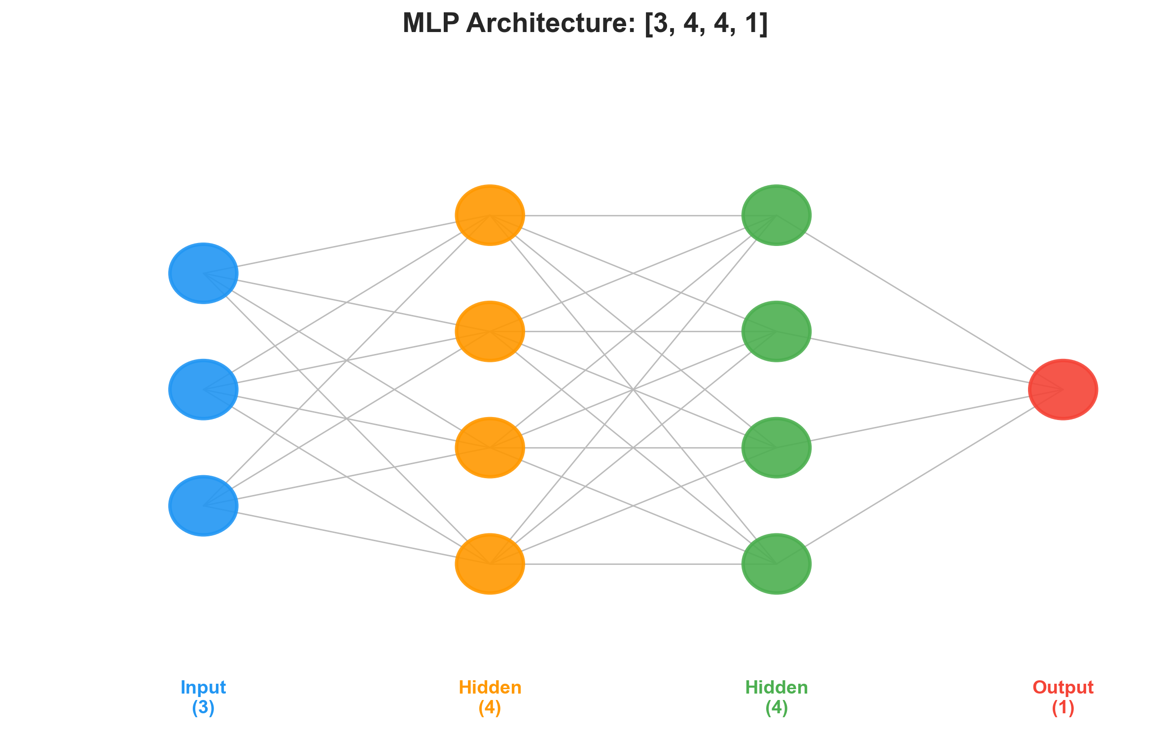
        return [p for layer in self.layers for p in layer.parameters()]

A network with two hidden layers of 4 neurons and a single output neuron:

n = MLP(3, [4, 4, 1])

This creates 41 trainable parameters (weights and biases across three layers). A forward pass through it builds a computation graph with dozens of nodes — every weight, bias, multiply, add, and tanh is a Value in the DAG. Despite that, backward() differentiates the entire graph in one pass by walking the topological order.

Training

Training a neural network is a three-step loop, and after all the machinery we built, the loop itself is almost anticlimactic:

for epoch in range(20):
    # Forward pass
    ypred = [n(x) for x in xs]
    loss = sum((yp - yt)**2 for yt, yp in zip(ys, ypred))

    # Zero gradients, then backward pass
    for p in n.parameters():
        p.grad = 0.0
    loss.backward()

    # Update: step opposite to gradient direction
    for p in n.parameters():
        p.data += -0.05 * p.grad

    print(epoch, loss)

Three things about this loop that are worth pausing on.

Zeroing gradients is not optional. The backward pass accumulates gradients with +=, which is correct within a single pass (that is the whole lesson from the gradient accumulation bug). But between training steps, the old gradients are stale. If you skip p.grad = 0.0, the gradients compound across epochs and the updates become enormous. I left the zeroing out once during debugging, and the loss went to inf within four epochs. PyTorch wraps this in optimizer.zero_grad(), but the underlying requirement is the same.

The learning rate is a balancing act. At $\alpha = 0.05$, this toy problem converges smoothly. At $\alpha = 1.0$, the loss oscillated and diverged. At $\alpha = 0.0001$, it converged but took thousands of epochs. For four data points and 41 parameters, finding a good learning rate took about 30 seconds of trial and error. For real problems, this becomes one of the most consequential hyperparameter choices — which is why adaptive methods like Adam exist.

The computation graph is rebuilt every iteration. Each call to n(x) constructs a fresh DAG from the current parameter values. The old graph from the previous iteration is discarded (Python’s garbage collector handles the cleanup). If you tried to reuse the old graph after updating parameters, the graph would reference stale Value objects with outdated data. The graph is ephemeral; only the parameter values persist between steps.

Watching It Converge

On four data points with binary targets $\{+1, -1\}$, the network converges quickly:

Input	Target	After Training
[2.0, 3.0, -1.0]	1.0	0.982
[3.0, -1.0, 0.5]	-1.0	-0.986
[0.5, 1.0, 1.0]	-1.0	-0.982
[1.0, 1.0, -1.0]	1.0	0.979

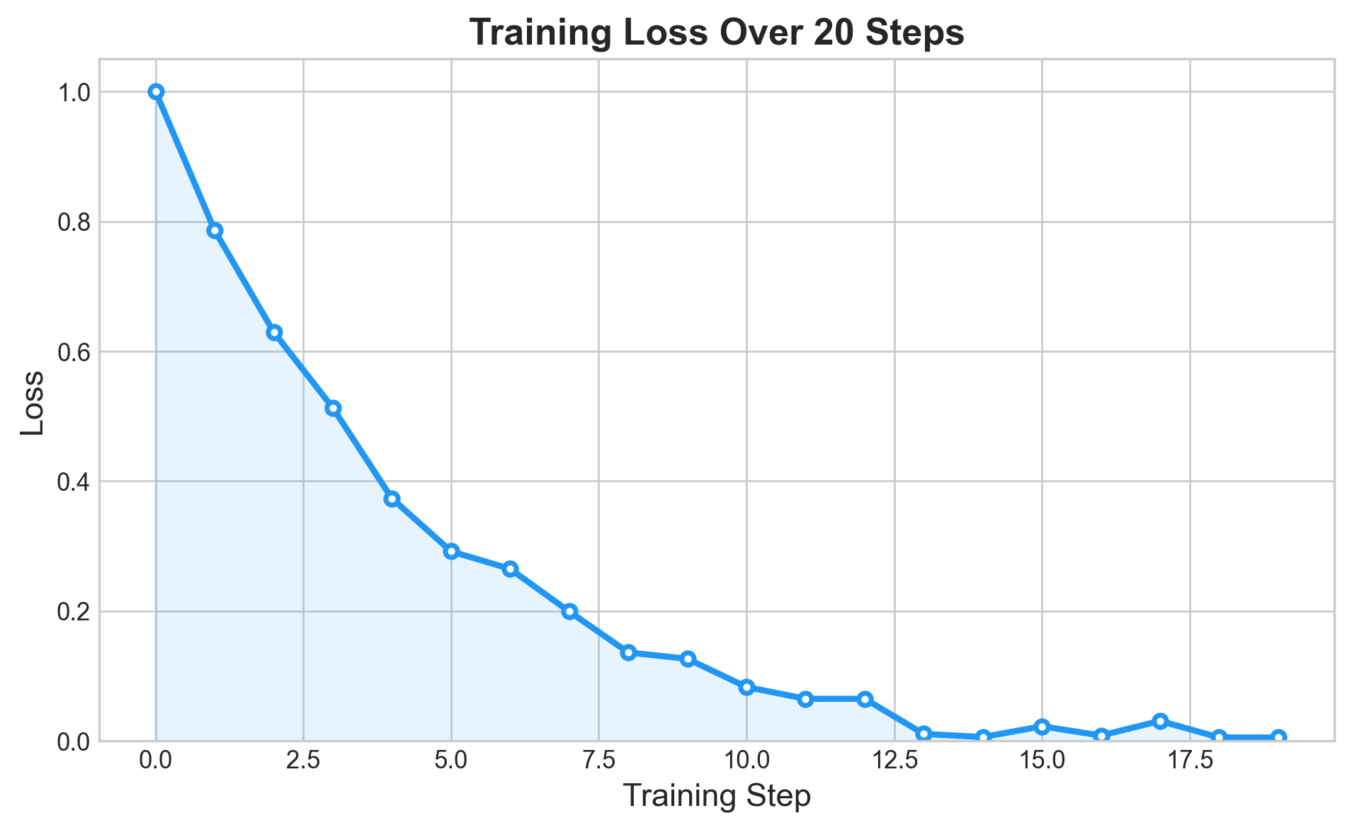
All predictions are within 0.02 of their targets. The network has memorized this tiny dataset, which is exactly what should happen when you have 41 parameters and 4 examples. Generalization is not the point here — verifying that the autograd engine supports end-to-end training is.

The training curve follows the textbook three-phase pattern. First, rapid descent: the randomly initialized predictions are far from the targets, gradients are large, and each step cuts the loss substantially. Then diminishing returns: as predictions approach the targets, $(y_{\text{pred}} - y_{\text{target}})$ shrinks, gradients shrink, and each step contributes less. Finally, convergence: the loss plateaus near zero. (With this problem and this architecture, “near zero” means around 0.001.)

What This Maps To in PyTorch

The training loop I wrote maps directly onto the standard PyTorch pattern:

# PyTorch equivalent
optimizer = torch.optim.SGD(model.parameters(), lr=0.05)

for epoch in range(20):
    ypred = model(x)
    loss = ((ypred - y)**2).sum()

    optimizer.zero_grad()  # our: p.grad = 0.0
    loss.backward()        # our: loss.backward()
    optimizer.step()       # our: p.data += -lr * p.grad

The structure is identical. PyTorch wraps gradient zeroing and parameter updates into an optimizer object, handles batching, supports GPU acceleration, and operates on tensors instead of scalars. The conceptual core — forward, backward, update — is the same three-step loop. The difference between this engine and PyTorch is scale and optimization, not concept.

What I Took Away

The complete Value class with all operations and the neural network abstractions together total under 100 lines of Python. There is something clarifying about the fact that the same algorithm running in PyTorch on GPU clusters with billions of parameters is, at its core, this: wrap your data in a structure that remembers how it was computed, attach a local gradient rule to each operation, sort the graph, walk backward. The rest is engineering.

Three specific things I did not fully understand before this project and do now:

Why gradient accumulation uses += and not =, and the class of bugs you get when you mix them up. The BUG-015 tanh issue was a direct instance of this, and finding it by staring at a computation graph for an hour taught me more about gradient flow than the relevant chapter in Goodfellow.

Why you zero gradients between training steps. The conceptual answer (“because backward accumulates”) is obvious once stated, but the operational consequence — that forgetting to zero turns your optimizer into a running sum of all past gradients, which blows up exponentially — is the kind of thing you remember after watching it happen.

Why the computation graph is rebuilt every iteration, and what would break if it were not. The graph encodes the specific computation that produced the current loss. After you update parameters, that computation is no longer the one you want to differentiate. A new forward pass with new parameter values requires a new graph.

For a more ambitious from-scratch project — a NumPy neural network trained on real image data — see Building a Neural Network from Scratch with NumPy .

---

The full source code, including the Graphviz visualization helpers, is available in the project repository .