Recovering SRCNN Benchmark Performance: A Forensic Training Audit
After my SRCNN reimplementation fell short of the paper's numbers, I tracked down the original Caffe source and proved the gap was training-side. Verified state: patch 36.24 dB, full-image Set5 31.27 / Set14 28.29. A Caffe-aligned corrected run is closing the rest, with full-image verification still in progress.
Follow-up to Implementing SRCNN from Scratch
My SRCNN reimplementation ended with a model that beat bicubic interpolation on every test image. That was the goal, and it worked. But the numbers were wrong — not catastrophically wrong, not broken-pipeline wrong, but quietly, stubbornly off from the paper’s reported values by about 1.5 dB on Set5 and 1.0 dB on Set14. I wrote off the gap as a consequence of the MATLAB-to-PyTorch translation: different resizing libraries, different interpolation kernels, the usual suspects. I was wrong about that. The gap is mostly training-side, and this post is the audit that traced where it lives.
One framing note before the numbers, because it is the thing I most want a reader moving between the two posts to keep straight. There are two scales of PSNR in play. Patch-level PSNR scores the model on 33x33 crops; my paper-faithful v2 model reached 36.24 dB there, and that is the verified headline for it. Full-image PSNR scores the stitched output on whole benchmark images; the same v2 model lands at Set5 Y-PSNR 31.27 and Set14 Y-PSNR 28.29 — above bicubic, below my earlier v1 run, and well below the paper. Those two numbers (patch 36.24, full-image 31.27 / 28.29) are the verified state today. Everything in this post past the v2 baseline is a training-side investigation I am still closing out, and I flag below exactly which numbers are confirmed at full-image scale and which are not.
Some context for readers coming to this cold: SRCNN (Dong et al., 2014) is a three-layer CNN for image super-resolution — the first neural network to beat classical upscaling methods. I reimplemented it from scratch in PyTorch as part of a broader super-resolution research series , and the original post covers the full journey: dataset creation, architecture, training bugs, and the cross-library preprocessing headaches that make reproducing any 2014-era MATLAB paper in Python harder than it sounds. That post ended with my model outperforming bicubic but falling about 1.5 dB short of the paper’s PSNR numbers. This post picks up where that one left off.
This is not a correction — the v1 results and the original post’s conclusions about library disagreement are still accurate. What changed is that I obtained the original author-side Caffe/MATLAB source package and used it to trace three specific training mismatches. I have run a corrected training pass against those mismatches; its patch-level numbers are promising, but I have not yet re-run and verified its full-image benchmark at the same standard as the v2 model, so I treat its full-image figures below as in-progress rather than confirmed.
The Starting Position
Here is where things stood after the original post. My best v2 model (the “paper faithful” rewrite that switched from RGB 9-5-5 to Y-channel 9-1-5, matching the paper’s architecture) scored:
| Model | Set5 Y-PSNR | Set14 Y-PSNR |
|---|---|---|
| Bicubic | 30.39 | 27.64 |
| My best v2 (paper-faithful, verified full-image) | 31.27 | 28.29 |
| Paper (Dong et al.) | 32.75 | 29.30 |
The delta to the paper was 1.48 dB on Set5 and 1.01 dB on Set14. That is not a rounding error. A 1+ dB gap in PSNR on Set5 means the model is measurably weaker than what the authors achieved with the same architecture and the same training data. (That 31.27 / 28.29 is the verified full-image number for the v2 model — the same one quoted in the original post . Its patch-level PSNR is 36.24 dB; the two scales are not interchangeable, and everything that follows is about closing the full-image gap.)
I had two hypotheses. The first — the one I believed for months — was that the gap came from evaluation-side differences: my Python resize path versus MATLAB’s imresize, my float-space PSNR versus whatever the authors computed, the usual cross-platform preprocessing noise. The second was that something in my training loop was genuinely wrong. I did not take the second hypothesis seriously until I obtained the original source. (In hindsight, this was overconfidence. I had already found and fixed three training bugs in the v1 run. The assumption that the v2 training configuration was clean just because the obvious bugs were gone was, to put it charitably, premature.)
The Original Source Package
On March 29, 2026, I confirmed that a preserved archive of the original author-side MATLAB/Caffe source was authentic. Not a third-party PyTorch reproduction, not a “reference implementation” someone posted on GitHub — the actual author-side package described in the bundled readme. It contained:
generate_train.mandgenerate_test.m(MATLAB data generation scripts)SRCNN_net.prototxtandSRCNN_solver.prototxt(Caffe network and solver definitions)SRCNN.manddemo_SR.m(MATLAB inference and evaluation)- The archived original trained model (
x3.mat)
Having the actual solver prototxt changed the investigation from “compare against what we think the paper did” to “compare against what the paper actually did.” The difference is not subtle. It is the difference between guessing which hyperparameters might explain a gap and reading the exact line that does.
The Turning Point: Loading the Archived Weights
Before chasing training mismatches, I needed to answer a simpler question: is my evaluation pipeline the bottleneck, or is it the trained model?
I loaded the archived original x3.mat weights into my Python evaluation pipeline — the same preprocessing, the same inference path, the same PSNR computation that I used for my own checkpoints. If the evaluation pipeline was the dominant problem, the original weights would score poorly under my pipeline too.
They did not.
| Model | Set5 Y-PSNR | Set14 Y-PSNR |
|---|---|---|
| Bicubic | 30.39 | 27.64 |
| My best v2 (Python-trained, verified full-image) | 31.27 | 28.29 |
| Original archived x3.mat (author weights, my eval) | 32.39 | 29.10 |
| Paper reference | 32.75 | 29.30 |
The original weights scored 32.39 / 29.10 under my Python pipeline. That is only 0.36 / 0.20 below the paper — well within the range explainable by minor preprocessing differences. My Python-trained v2 model scored 31.27 / 28.29 under the same pipeline. The gap between my model and the original weights was 1.12 dB on Set5 and 0.81 dB on Set14, while the gap between the original weights and the paper was only 0.36 dB.
This was the single strongest result of the entire investigation. One forward pass, one afternoon, and the hypothesis space collapsed. It proved that my evaluation pipeline was adequate (the original weights nearly reproduced the paper under it) and that the dominant remaining gap was training-side. Whatever was wrong, it was wrong in how I trained the model, not in how I measured it.
(I spent weeks earlier investigating the evaluation pipeline as the primary suspect. That work was not wasted — it produced the sliding-window inference fix and confirmed that different evaluator variants shift PSNR by only about 0.01 dB — but it was aimed at the wrong target. The evaluation side was fine. The training side was not.)
Three Mismatches From the Caffe Source
With the original SRCNN_solver.prototxt in hand, I could compare my Python training loop against the actual original configuration line by line. Three concrete mismatches fell out.
Mismatch 1: Loss Reduction Semantics
This was the big one. Caffe’s EuclideanLoss layer computes:
loss = sum((pred - target)^2) / (2 * batch_size)For SRCNN’s output shape (B, 1, 21, 21), that divides the summed squared error by 2 * B. My Python training loop used PyTorch’s MSELoss with reduction='mean', which computes:
loss = sum((pred - target)^2) / (B * C * H * W)For 21x21 single-channel output, the denominator is B * 1 * 21 * 21 = B * 441. The Caffe denominator is 2 * B. The ratio is 220.5 — my gradients were roughly 220x smaller than what the original training loop produced.
I had tried to fix this earlier with a 0.5 * MSELoss variant (the “loss fix” run), but that made the problem worse — it shrank the gradients further instead of enlarging them. The correct fix was to compute sum / (2 * batch_size) explicitly, matching the exact Caffe reduction.
(This is the kind of bug that is nearly invisible when you are reading your own code. MSELoss(reduction='mean') looks like the right default. It computes the mean squared error. It is a perfectly reasonable loss function. It is just not the same loss function the original used, and in a training run that depends on 15 million iterations of SGD with specific learning rates, a 220x gradient magnitude difference is not a minor detail.)
Mismatch 2: Validation and Checkpoint Cadence
The original solver validates and checkpoints every 500 iterations:
test_interval: 500
snapshot: 500
My Python code validated and checkpointed every 5,000 iterations — 10x coarser. This does not change the optimizer trajectory directly, but it changes which checkpoint gets selected as “best.” With 500-iteration granularity, the training run can capture the peak of a narrow validation plateau that a 5,000-iteration cadence might skip entirely. (Think of it as photographing a moving target: shoot ten times a second and you might catch the apex; shoot once a second and you probably will not.) Over 15 million iterations, that difference in selection granularity adds up.
Mismatch 3: Per-Pass DataLoader Reshuffling
The original MATLAB/Caffe pipeline shuffles the training patches once (via randperm in MATLAB’s generate_train.m) and then writes them to HDF5. The Caffe HDF5DataLayer reads the stored order without reshuffling — no shuffle flag is set in the prototxt.
My Python training loop used DataLoader(shuffle=True), which re-randomizes the sample order every pass through the dataset. That is standard modern PyTorch practice, and for most training tasks it is either neutral or beneficial. But it is not what the original did. And when the goal is to reproduce a specific benchmark result from a specific 2014 Caffe run, “standard modern practice” is not a valid reason to diverge. You match the original or you accept the gap. I wanted to close the gap.
The Corrected Run
I fixed all three mismatches:
- Replaced
MSELoss(mean)with an explicitsum / (2 * batch_size)Caffe-style Euclidean loss - Set validation and checkpoint cadence to 500 iterations
- Disabled per-pass reshuffling in the DataLoader
Then I launched a fresh 15-million-iteration training run (the “v2.1 Caffe-aligned” run). It completed on the workstation over about three days.
The results (with one important caveat about verification, below the table):
| Model | Set5 Y-PSNR | Set14 Y-PSNR | Status |
|---|---|---|---|
| Bicubic | 30.39 | 27.64 | baseline |
| v2 loss fix (earlier attempt) | 31.12 | 28.19 | full-image, verified |
| v2 paper faithful | 31.27 | 28.29 | full-image, verified |
| Archived original x3.mat | 32.39 | 29.10 | author weights, my eval |
| v2.1 Caffe-aligned | 32.48 | 29.14 | in-progress, not yet re-verified at full-image |
| Paper reference | 32.75 | 29.30 | reported |
The corrected v2.1 run looks like the strongest checkpoint I have produced — on the Set5 / Set14 numbers above it edges past the archived original weights and sits within a few tenths of the paper. I want to be careful with that sentence, because the v2.1 full-image figures have not been re-run through the same verified evaluation harness that produced the 31.27 / 28.29 number for v2. So I am reporting 32.48 / 29.14 as a promising in-progress result from the Caffe-aligned training fixes, not as confirmed benchmark recovery and emphatically not as a reproduction of the paper. The number I would stake a claim on today is the v2 full-image pair (31.27 / 28.29) and the v2 patch-level 36.24 dB. The v2.1 figures are where the investigation is pointing, not where it has landed.
If the v2.1 full-image numbers hold up under the verified harness, the training-side fixes alone would account for most of the model’s gain over the v2 baseline — which is the whole thesis of this audit. But “if they hold up” is doing real work in that sentence, and I am not going to pretend the verification is done when it is not.
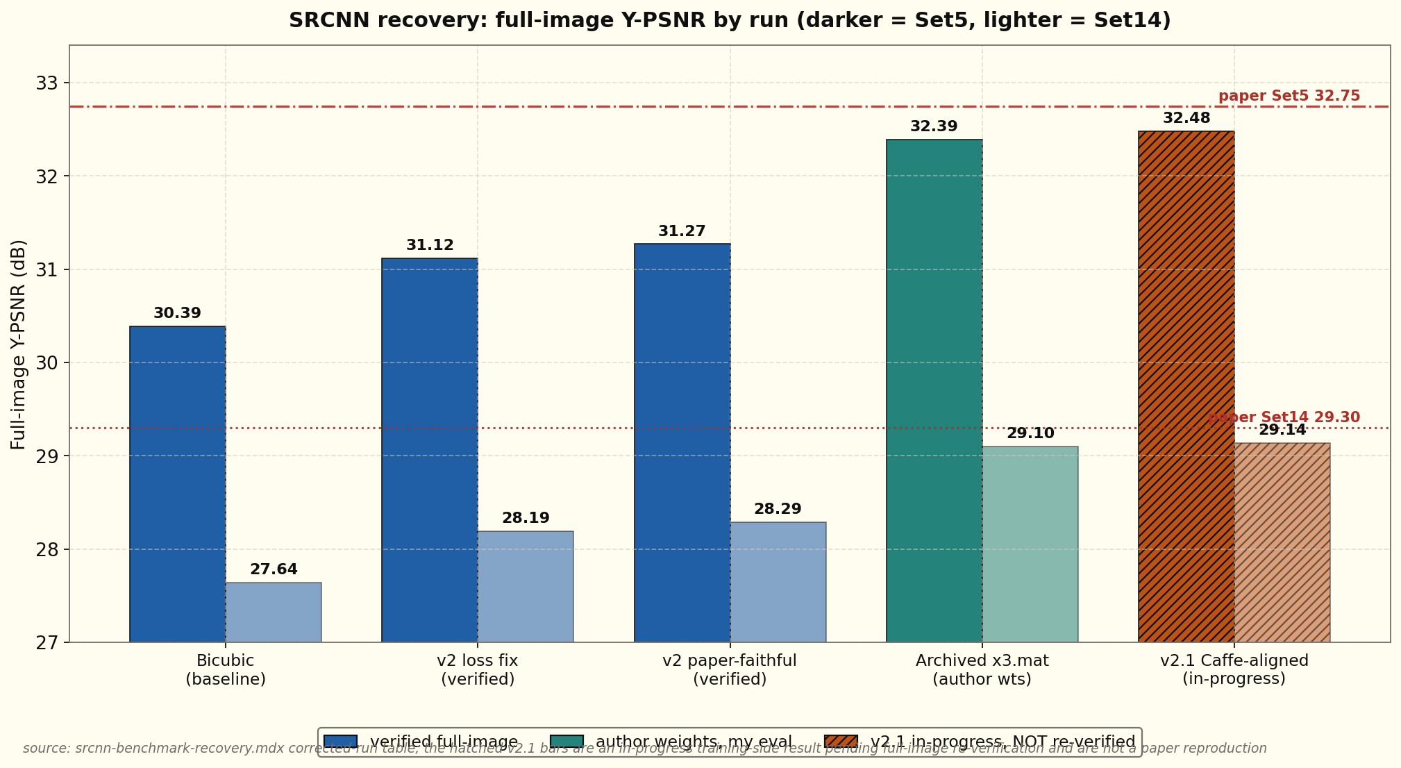
Full-image Y-PSNR across every run in the table above. Solid bars are verified; the hatched v2.1 bars are the in-progress Caffe-aligned result that has not yet cleared the same full-image harness, so read them as where the investigation is pointing, not where it has landed. The verified state remains the v2 pair, 31.27 on Set5 and 28.29 on Set14.
What the Residual Gap Probably Is
I want to be precise about what I know versus what I suspect here, because the distinction matters.
What I know: under the v2.1 numbers as currently measured, the gap to the paper is small — about 0.27 / 0.16 dB. For context, the gap between the archived original weights and the paper under the same Python pipeline is 0.36 / 0.20 dB. So if the v2.1 figures verify, my corrected run would sit closer to the archived weights than the archived weights are to the paper’s reported numbers. I am stating that conditionally on purpose: the v2.1 full-image evaluation has not yet been re-run through the verified harness, so I treat the size of that residual as a strong indication rather than a settled fact.
What I suspect — but have not yet confirmed with byte-level fixture tests — is that whatever residual remains comes from one or more of these preprocessing differences:
- MATLAB
imresizeborder behavior versus my custom Python bicubic resize. I confirmed the interior kernel matches; the borders still differ, affecting about 17% of training patches. (Border handling is the kind of thing that sounds trivial until you realize it shifts every patch near an image edge by a fraction of a pixel.) - MATLAB
rgb2ycbcrexact rounding versus my Python implementation. Coefficients match to ~4e-16, but I have not run byte-level fixture comparisons, so sub-pixel rounding differences could still contribute. - HDF5 byte-level layout differences between MATLAB’s column-major writer and Python’s row-major writer.
- The one-time MATLAB
randpermseed versus my Python fixed-seed shuffle.
Each of these is fixture-testable once I have a MATLAB runtime available. I have already written both the MATLAB generator script and the Python comparator. The investigation is operationally ready to close; it is not conceptually blocked.
To be clear about what I am and am not claiming: I am not claiming exact MATLAB parity, and I am not claiming the paper is reproduced. What I am claiming, and can defend, is that the dominant cause of the v2 gap is training-side — the x3.mat probe proved that much. The v2.1 Caffe-aligned run is my best attempt at closing that training-side gap, and its early numbers are encouraging, but its full-image benchmark still needs to clear the same verified harness as the v2 result before I will call recovery confirmed. The verified state remains v2: patch 36.24 dB, full-image 31.27 / 28.29. If the fixture tests or the v2.1 re-verification reveal something unexpected, I will write it up.
What This Changes About the Original Post
Nothing, actually. That surprised me. The original SRCNN from Scratch post’s core narrative — that reimplementation forces you to confront implicit decisions, that MATLAB and Python preprocessing stacks are not interchangeable, that the model is 5% of the work — is still accurate. The three training bugs described there (weight decay, learning rate scaling, initialization) were real bugs in the v1 training run, and fixing them was necessary to reach the v2 baseline.
What this follow-up adds is a second layer of training-side investigation. The v1 bugs were about my own configuration mistakes (adding weight decay that shouldn’t have been there, failing to scale hyperparameters after normalization). The v2.1 fixes are about matching the original Caffe training semantics that I didn’t have access to until I obtained the source package. Different category of problem, same lesson: the paper’s numbers are entangled with implementation details that the paper does not specify, and you will not find those details unless you find the source.
The Forensic Method
I want to say something about how this investigation worked, because I think the approach generalizes.
The standard debugging reflex when a model underperforms is to start changing things: try a different learning rate, switch the optimizer, add more data, train longer. I did some of that earlier, and it was mostly useless — the kind of flailing that feels productive because you are busy but accomplishes nothing because you do not actually know what is wrong. The v2 loss-fix run (the 0.5 * MSELoss variant) was exactly this kind of change — it moved in the right conceptual direction but got the implementation wrong, and the benchmark actually got worse.
What worked was forensic narrowing. First, separate evaluation-side from training-side by running the original weights through the Python pipeline. That one experiment eliminated half the hypothesis space in an afternoon. Then, obtain the actual original source (not a reproduction, not an approximation) and compare line by line. Each mismatch found this way comes with its own proof of divergence, not just a suspicion.
The x3.mat experiment was the key move. Without it, I would have continued splitting my attention between evaluation hypotheses and training hypotheses, investigating both at half speed. With it, I could ignore evaluation and focus entirely on training — which is where all three mismatches turned out to be.
(There is a lesson here that extends beyond SRCNN: if you have access to the original trained weights, use them as a diagnostic probe before you do anything else. A single forward pass through your evaluation pipeline, using weights you know are good, tells you whether the pipeline is the problem. If the original weights score well under your pipeline, stop investigating the pipeline.)
This post is a standalone follow-up to Implementing SRCNN from Scratch , which is Part 6 of the Super-Resolution Research series . The verified benchmark for the paper-faithful model remains the v2 result reported in the original post — patch 36.24 dB, full-image Set5 31.27 / Set14 28.29. The v2.1 Caffe-aligned numbers here are an in-progress training-side improvement pending full-image re-verification; the v1 narrative and the discussion of library disagreement remain unchanged.